RKNN2 SDK V2.5.0 · Quantization, hybrid quantization and QAT

Platform reference: this article follows the Rockchip RKNN2 SDK V2.5.0 Development Guide, including only the SoCs, Linux/Android Runtime and Toolkit combinations stated by the source. Features apply under the chip, SDK, driver and kernel conditions in each section, not automatically to every ArmSoM board. Check the actual ArmSoM BSP, NPU driver, Runtime and model versions before deployment. No ArmSoM hardware validation was performed; logs, performance figures and examples belong to the source.

Sources and proofreading: Chinese follows Chinese V2.5.0 (182 pages); English, Russian and German follow English V2.5.0 (208 pages). Source-specific technical information is retained; older-version content is not presented as new-version fact. Chinese figures come from the Chinese PDF; EN/RU/DE figures come from the English PDF, including separately extracted vector flowcharts. Original section and equation numbers remain. Some source cross-references still use old chapter numbers; dynamic-shape capacity examples contain “1224+140=264”, TP_NORM support statements conflict, and names such as init()/rknn.val_perf() differ from later API descriptions. These source issues are retained and require checking against actual V2.5.0 SDK headers/API references before execution. Code and parameters remain; PDF wrapping and table continuations are repaired.

Rockchip RKNN2 SDK V2.5.0

RKNN2 SDK V2.5.0 · 5/22

1. Software stack and core concepts

2. Environment, versions and board connection

3. Development workflow and interface selection

4. Model conversion and ONNX editing

Quantization, hybrid quantization and QAT

6. Inference, accuracy, performance and memory evaluation

7. Runtime lifecycle, layouts and memory

8. Zero-copy interfaces and I/O constraints

9. C API deployment and code generation

10. Toolkit Lite2 Python deployment

11. Matmul API and matrix layouts

12. NPU multicore configuration and performance

13. Dynamic-shape models and deployment

14. Multi-batch inference

15. RK3588/RK3576 NPU SRAM

16. Cache coherency and sparse inference

17. Custom operators: Python and C API

18. Encrypted model deployment

19. Accuracy troubleshooting

20. Performance analysis and network optimization

21. Memory analysis, sharing and reuse

22. FAQ, error handling and references

2.2 Model Quantization

2.2.1 Basic Concepts of Quantization

2.2.1.1 QUANTIZATION DEFINITION

Model quantization refers to converting the floating-point parameters or activation values of a deep learning model into fixed-point representations, such as converting FP32 to INT8. Quantization reduces memory usage and enables model compression and inference acceleration, but it usually introduces a certain degree of accuracy loss.

According to the form of the mapping function between floating-point values and fixed-point numbers, quantization can be divided into linear quantization and non-linear quantization. Common non-linear quantization methods include exponential quantization, codebook quantization, and piecewise linear quantization. RKNN-Toolkit2 supports linear quantization only. In linear quantization, the intervals between fixed-point numbers are uniform; for example, INT8 linear quantization divides the quantization range evenly into 256 values, which is why it is also called uniform quantization. According to whether the quantization zero point is 0, linear quantization can be divided into symmetric quantization and asymmetric quantization. Symmetric quantization is a simplified form of asymmetric quantization; asymmetric quantization usually handles non-uniform data distributions better, so asymmetric quantization is more commonly used in practice.

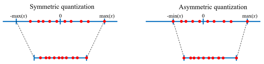
Figure 2-2 Linear Symmetric Quantization and Linear Asymmetric Quantization

2.2.1.2 QUANTIZATION CALCULATION

Taking linear asymmetric quantization as an example, the calculation of quantizing a floating- point number to a signed fixed-point number is as follows:

x_int = clamp(round(x / s) + z; -2^(b-1), 2^(b-1)-1)  (6-1)

where $x is the floating-point number, x int is the quantized fixed-point number, ⌊⋅⌉ is the round- to-nearest operation, s is the quantization scale factor, z is the quantization zero point, and b is the quantization bit width, e.g. b is 8 for the INT8 data type; clamp$ is the truncation operation, defined as follows:

clamp(x; a, c) = a, if x < a; x, if a <= x <= c; c, if x > c.  (6-2)

Converting a fixed-point number back to a floating-point number is called dequantization, defined as follows:

x ≈ x_hat = s × (x_int - z)  (6-3)

where xˆ is also called the pseudo-quantized floating-point number. It is easy to see that, due to the rounding and truncation operations in the quantization calculation, xˆ is not exactly equal to x ; the difference between them is called the quantization error.

Let the quantization range be $(q min ,q max ) and the truncation range be (c min ,c max ). The quantization parameters s and z$ are calculated as follows:

s = (q_max - q_min) / (c_max - c_min) = (q_max - q_min) / (2^b - 1)  (6-4)

z = c_max - round(q_max / s) OR z = c_min - round(q_min / s)  (6-5)

where the truncation range is determined by the quantized data type; for example, the truncation range of INT8 is (-128, 127). The quantization range is determined by the specific quantization algorithm. Setting z=0 in the above definitions yields the calculation definition of linear symmetric quantization.

2.2.1.3 QUANTIZATION GRANULARITY

Quantization granularity defines which parameters in a model’s floating-point tensor are quantized as a whole. RKNN-Toolkit2 supports three quantization granularities: Per-Layer / Per- Channel / Group. Per-Layer quantization quantizes all channels of a layer’s weights or activations as a whole, with all channels sharing the same quantization parameters. Per-Channel quantization quantizes each output channel of a layer’s weights independently, with each channel having its own quantization parameters. Group quantization applies only to linear-layer weights; on top of Per-Channel quantization, the elements of each output channel are split into groups, and each group is quantized independently.

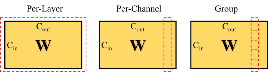
Figure 2-3 Per-Layer, Per-Channel and Group quantization

Note: In RKNN-Toolkit2, both Group and Per-Channel quantization apply to weights only; activations and intermediate values still use Per-Layer quantization. Group quantization is only valid for linear layers under w4a16.

2.2.1.4 QUANTIZATION ALGORITHMS

A quantization algorithm is a scheme for solving the mapping from floating-point tensors to low- bit fixed-point representations and their quantization parameters under a given quantization form (e.g. linear quantization). By implementation, they fall into two categories: quantization- aware training and post-training quantization. Quantization-aware training fine-tunes model and quantization parameters during training to improve accuracy; it usually requires deep understanding of the training pipeline and a large amount of training data, and is therefore rarely used directly in model deployment toolchains. Post-training quantization usually requires only a small calibration dataset, or even none, and obtains quantization parameters at low cost. RKNN- Toolkit2 supports four post-training quantization algorithms: Normal / KL-Divergence / MMSE and GDQ.

2.2.2 Overview of the Quantization Process

RKNN-Toolkit2 uses post-training quantization (PTQ): quantization is completed together with model conversion, via the internal quantization process. The floating-point model is first loaded into the Toolkit, and quantization is performed and the RKNN model exported through rknn.config() ──▶ rknn.load_xxx() ──▶ rknn.build() ──▶ rknn.export_rknn() . The overall quantization process is:

Floating-point model ──▶ rknn.config() to configure quantization parameters ──▶
rknn.load_xxx() to load the model ──▶ rknn.build(do_quantization=True, dataset=...)
to quantize and build ──▶ rknn.export_rknn() to export the RKNN model

The key elements of the quantization process and where they are configured:

Quantization data type: configured via quantized_dtype of rknn.config() ; RKNN- Toolkit2 supports w8a8, w4a16, w8a16 and other quantization data types (see 2.2.3.1 Data Types).

Quantization algorithm: configured via quantized_algorithm of rknn.config() ; four post-training quantization algorithms are supported: Normal / KL-Divergence / MMSE / GDQ (principles in 2.2.1.4 Quantization Algorithms, details in 2.2.3.2 Internal Quantization Algorithms).

Quantization granularity: configured via quantized_method of rknn.config() ; three granularities are supported: layer (Per-Layer) / channel (Per-Channel) / group{SIZE} (Group).

Quantization calibration set: specified via the dataset parameter of rknn.build() , used to compute the quantization parameters of activations (see 2.2.3.3 Calibration Data Preparation).

Hybrid quantization: assigns higher-precision data types to quantization-sensitive layers to mitigate accuracy loss (see 2.2.4 Hybrid Quantization).

Quantization-aware training (QAT): inserts fake-quantization nodes during training and fine-tunes model parameters; suitable for scenarios where post-training quantization cannot meet accuracy requirements (see 2.2.5 Quantization-Aware Training).

2.2.3 Internal Quantization Process

2.2.3.1 DATA TYPES

The quantization data types supported by RKNN-Toolkit2 internal quantization are w8a8 , w4a16 , w8a16 , w4a8 , w16a16i and w16a16i_dfp , with a default value of w8a8 . w4/w8/w16 means the weights are quantized to the corresponding bit width (int4/int8/int16), and a8/a16 means the activations are quantized to int8/float16. The quantization data types are described as follows:

w8a8 (default): weights in 8-bit asymmetric quantized precision, activations in 8-bit asymmetric quantized precision. Not supported on RK2118.

w4a16: weights in 4-bit asymmetric quantized precision, activations in 16-bit floating-point precision. Only supported on RK3576 / RV1126B.

w8a16: weights in 8-bit asymmetric quantized precision, activations in 16-bit floating-point precision. Only supported on RK3562.

w4a8: weights in 4-bit asymmetric quantized precision, activations in 8-bit asymmetric quantized precision. Not supported yet.

w16a16i: weights in 16-bit asymmetric quantized precision, activations in 16-bit asymmetric quantized precision. Only supported on RV1103 / RV1106.

w16a16i_dfp: weights in 16-bit dynamic fixed-point quantization precision, activations in 16-bit dynamic fixed-point quantization precision. Only supported on RV1103 / RV1106.

2.2.3.2 INTERNAL QUANTIZATION ALGORITHMS

Internal quantization supports four quantization algorithms: Normal / KL-Divergence / MMSE / GDQ:

Normal: determines the quantization range directly from the maximum and minimum floating-point values. It introduces no clipping error but is sensitive to outliers; it is fast and suitable for general scenarios. The quantization range is computed as:

q_min = min V  (6-6)

q_max = max V  (6-7)

where V is the floating-point tensor.

KL-Divergence: determines the quantization range by comparing the distributions of floating-point and fixed-point values, adjusting thresholds and minimizing the KL divergence. It adapts better to non-uniform data distributions and mitigates the impact of a few outliers; slightly slower than Normal.

argmin_(q_min,q_max) H(Ψ(V), Ψ(V_int))  (6-8)

where H(⋅,⋅) is the KL divergence, Ψ(⋅) is the function mapping the data to a discrete distribution, and V int is the quantized fixed-point tensor.

MMSE: determines the quantization range by minimizing the mean-square error between floating-point values and dequantized floating-point values. It usually achieves higher accuracy but requires more computation; it is slower and has higher memory overhead. Compared with KL-Divergence, it often performs better in outlier scenarios.

argmin_(q_min,q_max) ||V - V_hat(q_min,q_max)||_F²  (6-9)

where Vˆ (q min , q max ) is the quantize-dequantize form of V, and ∥⋅∥ F is the Frobenius norm.

GDQ: only valid when quantized_dtype is w4a16 or w8a16; it can effectively improve the weight quantization accuracy of w4a16 and w8a16. The recommended quantization dataset size is more than 200 images. For details of the GDQ algorithm, refer to the 《03_RKNN2_Toolkit_Python_API_Reference_V2.5.0》manual.

It is recommended to use the Normal algorithm first; when quantization accuracy issues arise, try KL-Divergence, MMSE or GDQ. For w4a16 / w8a16 quantization, try the GDQ algorithm first.

2.2.3.3 CALIBRATION DATA PREPARATION

In the internal quantization process, the calibration dataset is used to compute the quantization range of activations. It should cover the different data distributions of the model’s real application scenarios; for example, the calibration dataset of a classification model should contain images of different categories from real scenarios. A calibration dataset of 20~200 images is generally recommended, adjustable according to the runtime of the quantization algorithm; when using the GDQ quantization algorithm, a calibration dataset of more than 200 images is recommended. For other quantization algorithms, increasing the calibration dataset size increases runtime but does not necessarily improve accuracy.

Internal quantization calibration data currently supports text file format: write the paths of calibration images (jpg or png) or npy files into a .txt file, one path per line:

a.jpg
b.jpg

For multiple inputs, separate the files of each input with spaces:

a0.jpg a1.jpg
b0.jpg b1.jpg

2.2.3.4 CONCRETE EXAMPLE

Example 1: ResNet50 internal quantization process example:

from rknn.api import RKNN

model_path = "resnet50-v2-7.onnx" ## Floating-point ONNX model exported in advance
output_path = 'resnet50-v2-7.rknn'
DATASET_PATH = '../../../datasets/imagenet/ILSVRC2012_img_val_samples/dataset_20.txt'

# Create RKNN object
rknn = RKNN(verbose=False)

# Pre-process config
print('--> Config model')
rknn.config(mean_values=[[255*0.485, 255*0.456, 255*0.406]],
           std_values=[[255*0.229, 255*0.224, 255*0.225]],
           target_platform="rk3588",
           quantized_dtype='w8a8', ## "w4a16", "w8a16" etc. are optional (subject to actual platform support)
           quantized_algorithm='normal', ## "MMSE", "KL-Divergence", "GDQ" are optional
           quantized_method='channel',)
print('done')

# Load model
print('--> Loading model')
ret = rknn.load_onnx(model=model_path, inputs=['data'], input_size_list=[[1, 3,
224, 224]])

if ret != 0:
    print('Load model failed!')
    exit(ret)
print('done')

# Build model
print('--> Building model')
ret = rknn.build(do_quantization=True, dataset=DATASET_PATH)
if ret != 0:
    print('Build model failed!')
    exit(ret)
print('done')

# Export rknn model
print('--> Export rknn model')
ret = rknn.export_rknn(output_path)
if ret != 0:
    print('Export rknn model failed!')
    exit(ret)
print('done')

2.2.4 Hybrid Quantization

Hybrid quantization applies different quantization data types to different layers of the model, using higher-precision data types to represent layers that are not suitable for quantization, thereby mitigating the accuracy loss caused by model quantization. However, hybrid quantization introduces additional overhead and requires the user to determine the quantization data type of each layer.

2.2.4.1 USAGE OF HYBRID QUANTIZATION

To achieve a better balance between performance and accuracy, RKNN-Toolkit2 provides a hybrid quantization feature. Users can manually specify whether each layer should be quantized based on the output results of accuracy analysis.

Currently, the hybrid quantization feature supports the following usages:

Change specified quantized layers to non-quantized layers, e.g. compute them in FLOAT16. (Because non-quantized compute power on the NPU is lower, the inference speed will decrease to some extent.)
The quantization parameters of each layer can also be modified. (Modifying quantization parameters is not recommended.)

2.2.4.2 PROCESS OF HYBRID QUANTIZATION USAGE

When using the hybrid quantization feature, it involves four specific steps.

Load the original model and generate the quantization configuration file, temporary model file and data file. The specific interface calling process is as follows:

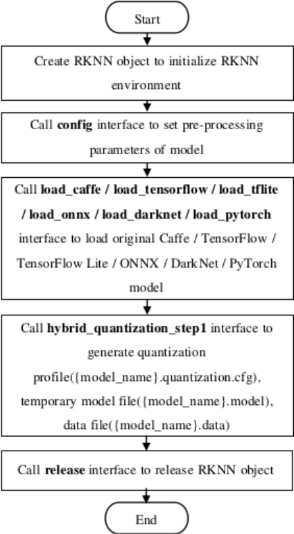
Figure 2-4 Hybrid quantization step 1

Modify the quantization configuration file generated in the first step.

After calling the hybrid_quantization_step1 interface in the first step, a configuration file named {model_name}.quantization.cfg will be generated in the current directory. The format of the configuration file is as follows:

custom_quantize_layers:
  Conv__350:0: float16
  Conv__358:0: float16
  ....
quantize_parameters:
  ....
  FeatureExtractor/MobilenetV2/Conv/Relu6:0:
    qtype: asymmetric_quantized
    qmethod: layer
    dtype: int8
    min:
    - 0.0
    max:
    - 6.0
    scale:
    - 0.023529411764705882
    zero_point:
    - -128
  ....

In the “custom_quantize_layers” section, users can add custom quantization layers by specifying the tensor name followed by the quantization type. This will change the operation type of the corresponding layer to the specified type. Currently, the available quantization data type is “float16”.

The “quantize_parameters” section contains the quantization parameters for each tensor in the model. The quantization parameters for each tensor are presented in the format of “tensor_name: quantization_properties_and_parameters”. The “min” and “max” represent the minimum and maximum values of the quantization range. Users can refer to the output results of precision analysis or use Netron to open the temporary model file named {model_name}.model to view the corresponding output tensor names.

Generate the RKNN model. The specific interface calling process is as follows:

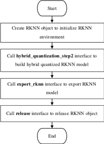
Figure 2-5 Hybrid quantization step 3

Perform inference using the RKNN model generated in the third step.

Note: In the RKNN-Toolkit2 project, under the “examples/functions/hybrid_quant” directory, there is an example of hybrid quantization. Users can refer to this example to perform hybrid quantization.

2.2.4.3 AUTOMATIC HYBRID QUANTIZATION

To make hybrid quantization easier to use and to solve model overflow issues, RKNN-Toolkit2 provides an automatic hybrid quantization feature. Through the auto_hybrid interface, users can automatically adjust the hybrid quantization model based on Euclidean distance and cosine distance thresholds during model quantization; when the model is non-quantized, it checks layer by layer whether fp16 overflow occurs and converts the overflowing layers to int16 computation.

Currently, the automatic hybrid quantization feature supports the following usages:

During model quantization, the hybrid quantization model is automatically adjusted based on Euclidean distance and cosine distance thresholds. Currently, only automatic adjustment from int8 quantization to fp16 is supported.

ret = rknn.build(do_quantization=True, dataset='./dataset.txt', auto_hybrid=True)

The thresholds for cosine distance and Euclidean distance can be set through auto_hybrid_cos_thresh and auto_hybrid_euc_thresh in the config interface. The cosine distance threshold defaults to 0.98, and the Euclidean distance threshold is not enabled by default. That is, by default only operators whose cosine distance accuracy is below the specified threshold are converted to fp16, in which case the Euclidean distance threshold has no effect. When the Euclidean distance threshold is enabled, operators whose cosine distance is below the cosine distance threshold or whose Euclidean distance is above the Euclidean distance threshold are converted to fp16.

When the model is non-quantized, it checks layer by layer whether fp16 overflow occurs and converts the overflowing layers to int16 computation. In this case, a dataset needs to be provided to calculate the numerical range of each layer

ret = rknn.build(do_quantization=False, dataset='./dataset.txt', auto_hybrid=True)

The maximum and minimum values of each layer are calculated based on the given input. When the maximum or minimum value exceeds the upper or lower limit of fp16, the operators of the corresponding layer are converted to int16.

2.2.5 Quantization-Aware Training (QAT)

2.2.5.1 INTRODUCTION TO QAT

Quantization-Aware Training (QAT) is a training method aimed at addressing the accuracy loss issue in low-bit quantization. Low-bit quantization can result in accuracy loss because converting the value range from floating-point numbers to fixed-point numbers incurs precision loss. During QAT training, the quantization error is incorporated into the training loss function, allowing the training of a model with quantization parameters.

Contrasting with Post Training Quantization (PTQ) provided by RKNN-Toolkit2, the characteristics of these two quantization methods are as follows:

Quantization Method	Secondary training based on the original framework	Dataset	Adjust the weight parameters	Loss function	Performance
Post Training Quantization (PTQ)	No	Small amount of unlabeled data	No	Irrelevant	Optimal
Quantization- Aware Training (QAT)	Yes	Complete training dataset	Yes	Quantization loss is included in the training loss function.	When there are operators that do not support QAT, the performance is slightly weaker than PTQ.

2.2.5.2 QAT PRINCIPLE

During QAT training, all weights are stored and calculations are performed in floating-point format, which ensures that backpropagation functions properly and the model can be trained effectively. Unlike training a floating-point model, QAT inserts FakeQuantize modules at quantizable locations in the model to simulate precision loss when converting from floating-point numbers to fixed-point numbers. This allows the loss function to recognize and optimize the quantization, ensuring accurate inference results when the model is converted to a fixed-point model.

QAT training is widely used and supported by mainstream inference frameworks. Users can refer to the links below for more detailed usage instructions.

Pytorch - https://pytorch.org/blog/quantization-in-practice/#quantization-aware-training-qat

Paddle - https://paddleslim.readthedocs.io/zh-cn/develop/api_cn/dygraph/quanter/qat.html

Tensorflow - https://www.tensorflow.org/model_optimization/guide/quantization/training

2.2.5.3 QAT USAGE GUIDELINES

Since QAT requires additional training code, and the code of some open-source repositories may conflict with the QAT feature, it is recommended to consider using QAT training for model quantization only when both of the following conditions are met:

Perform quantization accuracy troubleshooting as described in Chapter 5.1 to confirm that the PTQ feature of RKNN does not meet the accuracy requirements.
Try hybrid quantization as described in Chapter 2.2.4 to confirm that the hybrid quantization feature of RKNN does not meet the accuracy and performance requirements.

2.2.5.4 QAT IMPLEMENTATION EXAMPLE AND CONFIGURATION INSTRUCTIONS

Here are the documentations for QAT features in various frameworks. Please refer to the official documentation for actual usage.

PyTorch: https://pytorch.org/docs/stable/quantization.html (PyTorch has multiple sets of quantization interfaces. RKNN currently supports quantized models generated from the FX interface, specifically the prepare_qat_fx interface and its associated interfaces.)

Paddle: https://www.paddlepaddle.org.cn/tutorials/projectdetail/3949129#anchor-14

TensorFlow: https://www.tensorflow.org/model_optimization/guide/quantization/training

Taking PyTorch as an example to demonstrate the process of implementing QAT and some important considerations.

# for 1.10 <= torch <= 1.13
import torch
class M(torch.nn.Module):
    def __init__(self):
        super().__init__()
        self.conv = torch.nn.Conv(3, 8, 3, 1)

    def forward(self, x):
        x = self.conv(x)
        return x

# initialize a floating point model
float_model = M().train()

from torch.quantization import quantize_fx, QConfig, FakeQuantize, MovingAverageMinMaxObserver, MovingAveragePerChannelMinMaxObserver

qconfig = QConfig(activation=FakeQuantize.with_args(observer=
        MovingAverageMinMaxObserver,
        quant_min=0,
        quant_max=255,
        reduce_range=False), # reudece_range -> the default is True

 weight=FakeQuantize.with_args(observer=
      MovingAveragePerChannelMinMaxObserver,
      quant_min=-128,
      quant_max=127,
      dtype=torch.qint8,
      qscheme=torch.per_channel_affine,
      #qscheme->the default is torch.per_channel_symmetric
      reduce_range=False))
qconfig_dict = {"": qconfig}
model_qat = quantize_fx.prepare_qat_fx(float_model, qconfig_dict)

# define the training loop for quantization aware training
def train_loop(model, train_data):
    model.train()
for image, target in data_loader:
    ...
# Run training
train_loop(model_qat, train_loop)

model_qat = quantize_fx.convert_fx(model_qat)

In the above code flow, except for the adjustments made to the qconfig configuration for RKNN hardware, all other operations are implemented according to the guidance provided in the official codes. There are two main modifications in the qconfig:

The activation quantization configuration specifies reduce_range as False. When reduce_range is False, the effective quantization range is from -128 to 127. When reduce_range is True, the effective quantization range is from -64 to 63, which results in poorer quantization performance. RKNN hardware supports reduce_range as False.

The weight quantization configuration specifies qscheme as torch.per_channel_affine. The default torch.per_channel_symmetric restricts zero_point to be fixed at 0, but RKNN hardware supports non-zero zero_point. Therefore, torch.per_channel_affine is chosen.

2.2.5.5 SUPPORTED OPERATORS IN QAT

Taking PyTorch as an example, during the QAT process, Conv and Linear operators with weight parameters are first quantized according to QAT rules. Then other operators are examined. If they meet the regular quantization rules, they will be quantized in regular quantization. If an operator does not meet the QAT and regular quantization rules, it will maintain the FP32 computation rule.

Different frameworks have different levels of support. Users can refer to the following links to find more detailed information about the supported quantization operators based on the framework and version they are using:

Pytorch: https://github.com/pytorch/pytorch/blob/main/torch/ao/quantization/quantization_mappings.py

Paddle: https://github.com/PaddlePaddle/Paddle/blob/86df789a567f1285101c57b6e3ada4b952c58f48/pyt hon/paddle/quantization/config.py

Tensorflow: https://www.tensorflow.org/model_optimization/api_docs/python/tfmot/quantization/keras/Quantiz eConfig

2.2.5.6 HANDLING OF FLOATING-POINT OPERATORS IN QAT MODEL

In a QAT model, when an operator cannot be quantized, floating-point computation is used for it. When such operators are converted to an RKNN model, there are two scenarios to consider.

Preceded and followed by quantizable operators:

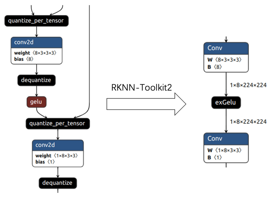
Figure 2-6 QAT OP preceded and followed by quantizable operators

As shown on the left of the figure above, the gelu operator in the original model is a floating- point operator, and the conv operators before and after it are quantized operators. When RKNN- Toolkit2 loads the model, it converts the floating-point operator between the two quantized operators into a quantized operator to improve inference performance, and this operation does not affect accuracy. After conversion to the RKNN model, the structure is as shown on the right of the figure above.

Non-quantizable operators exist before or after:

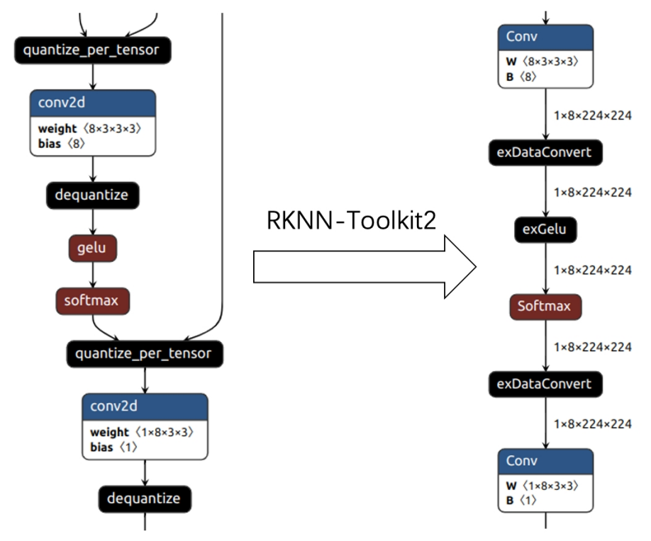
Figure 2-7 QAT OP preceded and followed by non-quantizable operators

As shown on the left of the figure above, the gelu and softmax operators in the original model are floating-point operators, and the conv operators before and after them are quantized operators. When RKNN-Toolkit2 loads the model, because the quantization parameters for gelu and softmax are missing, gelu and softmax remain in floating-point type. After conversion to the RKNN model, the structure is as shown on the right of the figure above: the RKNN model inserts a dequantization operator before gelu and a quantization operator after softmax, and these inserted quantization and dequantization operators all introduce additional time consumption.

2.2.5.7 SUMMARY OF QAT EXPERIENCE

QAT configuration

Depending on the characteristics of different hardware, QAT training often requires configuration adjustments to achieve better results. For RKNPU, it is recommended to configure the qconfig parameters by referring to the code instructions in 2.2.5.4 QAT Implementation Example and Configuration Instructions.

Quantization parameters saved in the model may require secondary adjustment

Take sigmoid as an example: the quantization parameters recorded by the sigmoid operator in the model may not be the ones actually used during inference. In the official code (https://github.com/pytorch/pytorch/blob/main/aten/src/ATen/native/quantized/cpu/qsigmoid.cpp), the quantization parameters of sigmoid are adjusted during inference, setting min to 0 and max to 1.

For such operators, RKNN-Toolkit2 adjusts their quantization parameters during the model conversion stage when converting QAT models, making the inference results closer to the original PyTorch inference results.