
Platform reference: this article follows the Rockchip RKNN2 SDK V2.5.0 Development Guide, including only the SoCs, Linux/Android Runtime and Toolkit combinations stated by the source. Features apply under the chip, SDK, driver and kernel conditions in each section, not automatically to every ArmSoM board. Check the actual ArmSoM BSP, NPU driver, Runtime and model versions before deployment. No ArmSoM hardware validation was performed; logs, performance figures and examples belong to the source.
Sources and proofreading: Chinese follows Chinese V2.5.0 (182 pages); English, Russian and German follow English V2.5.0 (208 pages). Source-specific technical information is retained; older-version content is not presented as new-version fact. Chinese figures come from the Chinese PDF; EN/RU/DE figures come from the English PDF, including separately extracted vector flowcharts. Original section and equation numbers remain. Some source cross-references still use old chapter numbers; dynamic-shape capacity examples contain “1224+140=264”, TP_NORM support statements conflict, and names such as init()/rknn.val_perf() differ from later API descriptions. These source issues are retained and require checking against actual V2.5.0 SDK headers/API references before execution. Code and parameters remain; PDF wrapping and table continuations are repaired.
RKNN2 SDK V2.5.0 · 4/22
1. Software stack and core concepts
2. Environment, versions and board connection
3. Development workflow and interface selection
Model conversion and ONNX editing
5. Quantization, hybrid quantization and QAT
6. Inference, accuracy, performance and memory evaluation
7. Runtime lifecycle, layouts and memory
8. Zero-copy interfaces and I/O constraints
9. C API deployment and code generation
10. Toolkit Lite2 Python deployment
11. Matmul API and matrix layouts
12. NPU multicore configuration and performance
13. Dynamic-shape models and deployment
16. Cache coherency and sparse inference
17. Custom operators: Python and C API
18. Encrypted model deployment
20. Performance analysis and network optimization
21. Memory analysis, sharing and reuse
22. FAQ, error handling and references
2. Model Conversion, Quantization, and Evaluation
2.1 General Model Conversion
RKNN-Toolkit2 provides rich functionality, including model conversion, performance analysis, deployment and debugging, etc. This section focuses on the model conversion function of RKNN- Toolkit2. Model conversion is one of the core functions of RKNN-Toolkit2. It allows users to convert deep learning models from various frameworks into RKNN format to run on RKNPU. The overall workflow is: model preparation → configuration of conversion parameters → loading and building the model → exporting the RKNN model → verifying the conversion result. Users can refer to the following model conversion flow chart to understand how to perform model conversion.
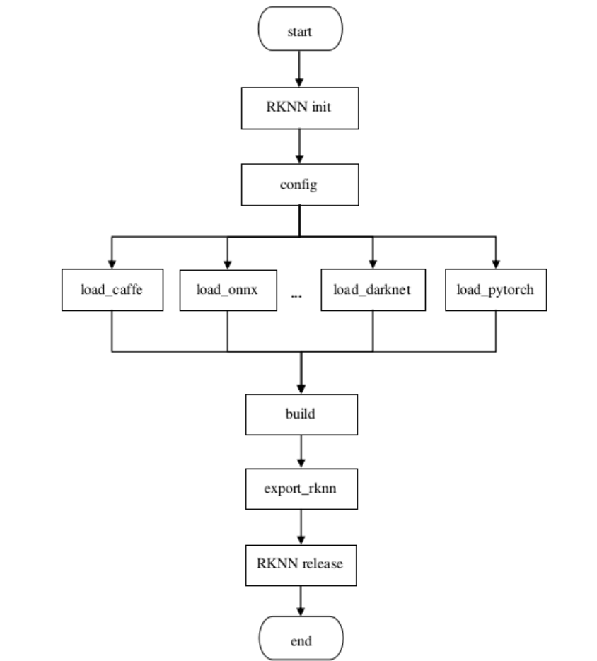
Figure 2-1 The flow chart of model conversion
Currently RKNN-Toolkit2 supports model conversion for multiple popular deep learning frameworks, including:
Caffe
TensorFlow
TensorFlow Lite
ONNX
PyTorch
Darknet
Users can use the above frameworks to train or obtain pre-trained models and convert them into RKNN format, making it easier and more efficient to deploy and run inference on the RKNPU platform.
2.1.1 Model Preparation
The input of model conversion is the original model trained or exported from each deep learning framework. Complete the following preparations before conversion:
Model source: use a pre-trained model trained or obtained from a framework supported by RKNN-Toolkit2 (Caffe / TensorFlow / TensorFlow Lite / ONNX / PyTorch / DarkNet), and make sure the model infers correctly in the original framework.
Input/output information: identify the model’s input/output node names, input shapes, data types, etc. Some frameworks require this information explicitly when loading (e.g. TensorFlow’s inputs / outputs / input_size_list, PyTorch’s input_size_list); the subsequent configuration and loading APIs will use it.
Model check: before conversion, it is recommended to inspect the model structure with tools such as Netron to confirm the model was exported correctly and its operators are supported; for ONNX models, onnxruntime can be used first to verify that the inference results match the original framework.
2.1.2 Conversion Configuration
Before model conversion, users need to set some configurations to ensure the correctness and performance of model conversion. Configuration parameters can be set through the rknn.config() interface, including setting the input mean, normalized value, whether to quantize, etc. Some commonly used configuration parameters are listed below:
mean_values and std_values are used to set the mean and normalized values of the input. These values are used in the quantification process, and the images no longer need to be averaged and normalized during the C API inferencing to reduce deployment time.
quant_img_RGB2BGR is used to control whether RGB to BGR conversion needs to be performed first when loading a quantization image during quantization. The default value is false. This configuration takes effect during quantification correction and will not take effect during the model inference stage. It needs to be processed by the users in pre-input processing. Please refer to Chapter 5.4.3 for detailed precautions. Note: Note: When quant_img_RGB2BGR= True, the model’s inference sequence is to perform RGB2BGR conversion first then perform mean_valuesand std_values operations later.
target_platform is used to specify the target platform of the RKNN model, supporting RV1103, RV1103B, RV1106, RV1106B, RV1126B, RK2118, RK3562, RK3566, RK3568, RK3576 and RK3588 at the moment.
quantized_algorithm is used to specify the quantization algorithm used when calculating the quantized parameters of each layer. You can choose normal, mmse, kl_divergence or gdq. The default algorithm is normal. For detailed description, see chapters 3.1.7, 6.1 and 6.2.
quantized_method supports layer, channel or group{SIZE}, used to determine whether the weights of each layer share parameters. The default is channel. For details, see chapters 3.1.7, 6.1 and 6.2.
optimization_level is used to modifying the model optimization level, you can turn off some or all of the optimization rules used in the model conversion process. The default value of this parameter is 3, which turns on all optimization options. When the value is 2 or 1, some optimization options that may affect the accuracy of some models are turned off. When the value is 0, all optimization options are turned off.
quantized_dtype is used to specify the quantization type. Currently, INT8 for linear asymmetric quantization is supported, and the default is ‘asymmetric_quantized-8’.
custom_string is used to adds custom string information to the RKNN model, such as version information of the model`s own iteration, etc. This information can be obtained by querying RKNN_QUERY_CUSTOM_STRING which facilitates special processing according to different RKNN models during deployment. The default value is None.
dynamic_input supports dynamic input and simulates the function of dynamic input according to multiple sets of input shapes specified by the users. The default value is None. See Chapter 4.1.3 for details.
For more specification of rknn.config(), please refer to the 《03_RKNN2_Toolkit_Python_API_Reference_V2.5.0》manual. Only some common parameters are listed above.
Example code:
rknn.config(
    mean_values=[[103.94, 116.78, 123.68]],
    std_values=[[58.82, 58.82, 58.82]],
    quant_img_RGB2BGR=False,
    target_platform='rk3566')
2.1.3 Model Loading and Building
1. Initialize the RKNN object
In this stage, users need to initialize the RKNN object first, which is the first step of the entire workflow:
Use the RKNN() constructor to initialize the RKNN object. Users can pass in the parameters verbose and verbose_file .
The verbose parameter determines whether to display detailed log information on the screen.
If the verbose_file parameter is set and verbose is True , the log information will also be written to the specified file.
Example code:
rknn = RKNN(verbose=True, verbose_file='./mobilenet_build.log')
2. Model loading interfaces
Users need to use the corresponding loading interface to import model files from different frameworks. RKNN-Toolkit2 provides different loading interfaces, including Caffe, TensorFlow, TensorFlow Lite, ONNX, PyTorch, etc. The following is a brief introduction to the model loading interfaces of each framework:
Caffe model loading interface:
Use the rknn.load_caffe() interface to load a Caffe model.
You need to provide the model file ( .prototxt suffix) path and the weight file ( .caffemodel suffix) path.
If the model has multiple input layers, you can specify the order of the input layer names.
Example code:
ret = rknn.load_caffe(model='./mobilenet_v2.prototxt', blobs='./mobilenet_v2.caffemodel')
TensorFlow model loading interface:
Use the rknn.load_tensorflow() interface to load a TensorFlow model.
You need to provide the TensorFlow model file ( .pb suffix) path, the input node names, the input node shapes, and the output node names.
Example code:
ret = rknn.load_tensorflow(tf_pb='./ssd_mobilenet_v1_coco_2017_11_17.pb',
              inputs=['Preprocessor/sub'],
              outputs=['concat', 'concat_1'],
              input_size_list=[[1, 300, 300, 3]])
TensorFlow Lite model loading interface:
Use the rknn.load_tflite() interface to load a TensorFlow Lite model.
You need to provide the TensorFlow Lite model file (.tflite suffix) path.
Example code:
ret = rknn.load_tflite(model='./mobilenet_v1.tflite')
- ONNX model loading interface: - Use the rknn.load_onnx() interface to load an ONNX model. - You need to provide the ONNX model file (.onnx suffix) path.
Example code:
ret = rknn.load_onnx(model='./arcface.onnx')
DarkNet model loading interface:
Use the rknn.load_darknet() interface to load a DarkNet model.
You need to provide the DarkNet model file ( .cfg suffix) path and the weight file ( .weights suffix) path.
Example code:
ret = rknn.load_darknet(model='./yolov3-tiny.cfg', weight='./yolov3.weights')
- PyTorch model loading interface: - Use the rknn.load_pytorch() interface to load a PyTorch model. - You need to provide the PyTorch model file (.pt suffix) path, and the model must be in torchscript format.
Example code:
ret = rknn.load_pytorch(model='./resnet18.pt', input_size_list=[[1, 3, 224, 224]])
Users can select the appropriate interface to load models from different frameworks, so as to ensure the correctness of model conversion.
3. Build the RKNN model
After loading the original model, the next step is to build the RKNN model through the rknn.build() interface. When building a model, users can choose whether to perform quantization, which can reduce the model size and improve performance on RKNPU. The parameters of the rknn.build() interface are as follows:
do_quantization: this parameter controls whether to quantize the model. It is recommended to set it to True .
dataset: this parameter specifies the dataset used for quantization calibration. The format of the dataset is a text file.
Example of dataset.txt:
./imgs/ILSVRC2012_val_00000665.JPEG
./imgs/ILSVRC2012_val_00001123.JPEG
./imgs/ILSVRC2012_val_00001129.JPEG
./imgs/ILSVRC2012_val_00001284.JPEG
./imgs/ILSVRC2012_val_00003026.JPEG
./imgs/ILSVRC2012_val_00005276.JPEG
Example code:
ret = rknn.build(do_quantization=True, dataset='./dataset.txt')
2.1.4 Exporting the RKNN Model
After building the RKNN model through the rknn.build() interface, users can export the RKNN model file ( .rknn suffix) through the rknn.export_rknn() interface for subsequent model deployment. The parameters of the rknn.export_rknn() interface are as follows:
export_path: the path of the exported model file.
cpp_gen_cfg: this parameter determines whether to generate a C++ deployment example when exporting the model.
Example code:
ret = rknn.export_rknn(export_path='./mobilenet_v1.rknn')
After the conversion workflow is completed, call the release() interface to release the resources occupied by the RKNN object:
rknn.release()
2.1.5 Conversion Result Verification
After exporting the RKNN model, it is recommended to verify the conversion result:
Simulator inference verification: on the PC, run inference on the model with the simulator via rknn.init_runtime(target=None) ( rknn.inference() ), and compare the output with the inference result of the original model in the original framework (cosine distance can be used to check consistency) to confirm that no error was introduced during conversion.
Board-connected inference verification: connect the development board to the PC via USB and run board-connected inference via rknn.init_runtime(target=xxx) to verify the results on real NPU hardware.
Note: For more detailed evaluation methods such as accuracy analysis, performance evaluation, and memory evaluation, see 2.3 Model Evaluation.
2.1.6 Model Conversion Tool: rknn_convert
rknn_convert is a set of commonly used model conversion tools provided by RKNN-Toolkit2. By encapsulating the above API interfaces, users only need to edit the yml configuration file corresponding to the model to convert the model through a command. The following is an example command of how to use the rknn_convert tool and the supported command parameters:
python -m rknn.api.rknn_convert -t rk3588 -i ./model_config.yml -o ./output_path
By using the above commands and parameters, users can convert models into RKNN format and save the converted models to the specified output path. The supported command parameters are described as follows:
-i: the path of the model configuration file (.yml).
-o: the output path of the converted model.
-t: target_platform. The target platform can be rv1103, rv1103b, rv1106, rv1106b, rv1126b, rk2118, rk3562, rk3566, rk3568, rk3576 or rk3588.
-e: (Optional) Evaluate the time consumption and memory usage of the model during board- connected runtime. Enter -e to enable it. Note: Be sure to connect the corresponding development board and set target_platform correctly, otherwise an error will be reported. When there are multiple devices, use the -d parameter to specify the device ID.
-a: (Optional) Evaluate the accuracy of the generated rknn model. To enable simulator accuracy evaluation, enter -a “xx1.jpg xx2.jpg”. To enable board-connected accuracy evaluation, use it together with the -d parameter.
-v: (Optional) Specify whether to print detailed log information on the screen. Enter -v to enable printing mode.
-d: (Optional) Use -d for a single adb device, and -d device_id for multiple adb devices. Query device_id through adb devices.
The following is a reference yml configuration file ( object_detection.yml ):
models:
   # model output name
   name: object_detection
   # Original model framework
   platform: onnx
   # Model input file path
   model_file_path: ./object_detection.onnx
   # Describe information such as input and output shapes
   subgraphs:
     # model input tensor shape
     input_size_list:
       - 1,3,512,512
     # input tensor name
     inputs:
       - data
     # output tensor name
     outputs:
       - conv6-1
       - conv6-2
       - conv6-3
   # quantification flag
   quantize: true
   # Quantify dataset file path (relative yml path)
   dataset: ./dataset.txt
   configs:
     quantized_dtype: asymmetric_quantized-8
     # rknn.config mean_values
     mean_values: [127.5,127.5,127.5]
     # rknn.config std_values
     std_values: [128.0,128.0,128.0]
     # rknn.config quant_img_RGB2BGR
     quant_img_RGB2BGR: false
     # rknn.config quantized_algorithm
     quantized_algorithm: normal
This configuration file includes detailed information such as the model name, the framework used by the original model, the model file path, input and output information, and whether to perform quantization. Users can edit the corresponding configuration file according to the specific requirements of the model.
For the model conversion configuration, see the table below:
Table 2-1 Description of rknn_convert model conversion configuration parameters
| Parameter | Content to fill in |
|---|---|
| -name | Model output name |
| -platform | The framework used by the original model, supporting tensorflow, tflite, caffe, onnx, pytorch, darknet |
| -model_file_path | Original model file path, applicable to single model file input, e.g.: tensorflow, tflite, onnx, pytorch |
| -quantize | Whether to enable quantization |
| -dataset | The quantization dataset file path (relative to the yml configuration file path). This item is required if accuracy_analysis is enabled |
| -prototxt_file_path | When platform is caffe, the prototxt file of the model |
| -caffemodel_file_path | When platform is caffe, the caffemodel file of the model |
| -darknet_cfg_path | When platform is darknet, the cfg file of the model |
| -darknet_weights_path | When platform is darknet, the weight file of the model |
| -subgraphs | Describes information such as input and output shapes. Except for specific frameworks, this parameter and its sub-parameters generally do not need to be filled in, and the model default values are used |
| —-input_size_list | The shape of the input tensor (Subparameter) |
| —-inputs | (Subparameter) The name of the input tensor |
| —-outputs | (Subparameter) The name of the output tensor |
| -configs | The corresponding rknn.config() configuration |
| —-quantized_dtype | Quantization type. RKNN_toolkit2: can be set to [asymmetric_quantized-8]. (Subparameter) If not entered, the default value is used |
| —-mean_values | The mean normalization value of the input. For a single-input RGB model, (Subparameter) e.g., [123.675,116.28,103.53]; for multiple inputs, e.g., [[123,116,103], [255,255,255]] |
| —-std_values | The std normalization value of the input. For a single-input RGB model, e.g., (Subparameter) [58.395,58.295,58.391]; for multiple inputs, e.g., [[127,127,127], [255,255,255]] |
| —-quant_img_RGB2BGR | Controls whether the quantization calibration images need to be converted (Subparameter) from RGB to BGR first when loading them for quantization. The default value is False |
| —-quantized_algorithm | Quantization algorithm, selectable from [‘normal’, ‘kl_divergence’, ‘mmse’], (Subparameter) default is normal |
| —-quantized_method | Quantization method. RKNN_toolkit2 options are [‘layer’, ‘channel’], default (Subparameter) is channel |
| —-optimization_level | Sets the optimization level. The default is 3, which means using all default (Subparameter) optimization options |
| —-model_pruning | Prune the model to reduce the model size. Defaults to false; set to true to (Subparameter) enable |
| —-quantize_weight | When the quantize parameter is false, reduce the size of the rknn model by (Subparameter) quantizing some weights. Defaults to false; set to true to enable |
| —-single_core_mode | Whether to generate a single-core model only, which can reduce the size (Subparameter) and memory consumption of the RKNN model. The default value is False. Currently effective for RK3588/RK3576. The default value is False |
2.1.7 Quantization Feature of RKNN-Toolkit2
RKNN-Toolkit2 provides multiple quantization methods and multiple quantization algorithms, selected via the quantized_algorithm and quantized_method parameters in rknn.config(). This section describes the commonly used Normal / MMSE / KL-Divergence quantization algorithms and the Layer / Channel quantization methods; the GDQ quantization algorithm and the Group quantization method are described in 2.2.3 Internal Quantization Process. The following introduces these quantization algorithms and feature quantization methods:
Quantization algorithms:
Normal quantization algorithm: determines the maximum and minimum values of the quantization range directly from the maximum and minimum floating-point values of the model features (feature). It is fast, but performs poorly when the feature distribution is imbalanced. The recommended quantization dataset size is generally about 20-100 images.
MMSE quantization algorithm: determines the maximum and minimum values of the quantization range by minimizing the mean-square-error loss between floating-point values and quantize-dequantize floating-point values, which can alleviate the quantization accuracy loss caused by large outliers to a certain extent. It uses brute-force iteration and is slower, but usually achieves higher accuracy than normal. The recommended quantization dataset size is generally about 20-50 images, which can be adjusted according to the quantization time.
KL-Divergence quantization algorithm: abstracts the floating-point and fixed-point values of model features into two distributions, updates the distributions by adjusting thresholds, and determines the maximum and minimum values of the quantization range by measuring the similarity of the two distributions with KL divergence. It takes more time than normal but much less than mmse, and can achieve good improvement in some scenarios (uneven feature distribution). The recommended quantization dataset size is generally about 20-100 images.
Quantization methods:
Layer quantization method: quantizes all channels of the same network layer as a whole; all channels share the same quantization parameters.
Channel quantization method: quantizes each output channel of the same network layer independently; each channel has its own quantization parameters. Generally, the Channel method achieves higher accuracy than the Layer method.
According to the actual model quantization effect and requirements, users can choose a suitable quantization algorithm and feature quantization method. For more details on quantization, see Chapter 2.2 (Model Quantization).
GDQ quantization algorithm: only valid for w4a16 and w8a16; it can effectively improve the weight quantization accuracy of w4a16 and w8a16. The recommended quantization dataset size is more than 200 images. See 2.2.3.2 Internal Quantization Algorithms for details.
2.1.8 Model Pruning
Model pruning can generally be divided into two methods: lossy pruning and lossless pruning. The model pruning of RKNN-Toolkit2 is lossless pruning, which means that it can reduce the size of the model and the amount of calculation without degrading floating point accuracy of the model. And the quantization accuracy of the model can even be improved.
However, not all models can be used for lossless pruning. Lossless pruning is based on the degree of sparseness of the model’s weights to remove some weights and feature channels that have no impact on the model, results to reduce the size and the calculation of the model After the model pruning configuration is enabled (set the model_pruning parameter of rknn.config() to True), the model will be automatically pruned according to the degree of weight sparsification during model conversion.
If the model is pruned successfully, the results will be printed, as follows:
I model_pruning results:

I Weight: -1.12145 MB (-6.9%)

I GFLOPs: -0.15563 (-13.4%)
Among Weight cut off 1.12145 MB (accounting for 6.9%), and the model calculation was reduced by 0.15563 GFLOPs (accounting for 13.4%).
If pruning fails due to insufficient model sparsity, no processing will be done (nor will the above information be printed), so this configuration will not affect normal model conversion.
2.1.9 ONNX Model Editing
Some models may have redundant ops after being converted to the RKNN model. It is common for redundant reshape and transpose ops to exist at the input and output nodes of the model, which affects the inference performance of the RKNN model. RKNN-Toolkit2 provides the onnx_edit interface, which is used to modify the input and output dimension definitions of the ONNX model, so that the adjusted onnx model can be converted into a RKNN model with better performance and reduce redundant reshape and transpose ops.
2.1.9.1 INTERFACE DESCRIPTION
Usage example:
from rknn.utils import onnx_edit
ret = onnx_edit(model = './concat_block.onnx',
  export_path = './concat_block_edited.onnx',
  inputs_transform = {'k_in': 'a,b,c,d->1,ad,b,c'},
  outputs_transform = {'k_cache': 'a,b,c,d->1,ab,c,d'},
  dataset = './dataset.txt'
)
Model fills in the model to be modified, which is a required parameter.
Export_path fills in the generation path of the new model, which is a required parameter.
Inputs_transform fills in the transformation formula dictionary of the input node, the key is the node name, and the value is the transformation formula. It is an optional parameter and defaults to an empty dictionary.
Outputs_transform fills in the transformation formula dictionary of the output node. It is an optional parameter and defaults to an empty dictionary.
Dataset fills in the path set file of the input data. The file format requirements are consistent with the requirements of the rknn.build interface for dataset. After filling in, the onnx_edit interface will not only adjust the input and output definitions of the model, but also adjust the corresponding data in the dataset, and generate new dataset data in the directory at the same level as export_path, which can be used for verification and quantification of the new model. It is an optional parameter and is empty by default.
2.1.9.2 TRANSFORMATION FORMULA DESCRIPTION
The inputs_transform and outputs_transform in the onnx_edit interface need to be filled with transformation formulas. The definition of the transformation formula is similar to the definition of the einsum operator. For example, the ‘a,b,c,d->1,ad,b,c’ formula refers to transforming the original dimensions into ‘a,b,c,d’. followed by ‘1,ad,b,c’. The rules for filling in the transformation formula are as follows:
Must be composed of two parts of characters, separated by ‘->’. The left side is the original character shape, and the right side is the transformed character shape.
The symbols in the character shape are only allowed to be [a-z] or ‘,’ ‘1’. Except for ‘1’, other numeric shape characters are not supported. The reason is that the same numeric characters cannot determine the context of transpose.
Characters [a-z] are considered independent and have no sequential relationship, that is, ‘a,b->b,a’ and ‘c,a->a,c’ represent the same transformation
The original character shape on the left side of the equation is separated into n parts by ‘,’. The number of n must match the dimensions of the model. For example, the model input definition is [32,4,1,64], and the input character can be ‘a ,b,c,d’ or ‘a,b,1,d’
Every symbol of the original character shape, except ‘1’, must exist in the transformed character shape. For example, ‘a,1,c,d->ac,d,1’ is valid, ‘a,1,c,d->ac,1’ is invalid, ‘d’ is missing
The transformed character shape allows the insertion of any number of ‘1’s to achieve the dimension expansion effect, such as ‘a,b,c-> a,1,cb,1,1’
Original character shape allows multiple letters and assignment formulas to be used to express splitting the shape. For example, the original input definition is [32,4,1,64], ‘ab,c,d,qk[a=2,k =8]->aq,cd,1,kb’, which means split 32 into 2x16, split 64 into 8x8, and then perform transpose and reshape operations. The ‘[ ]’ part is called the assignment formula, and multiple formulas are separated by ‘,’ symbols. In addition, it is allowed that a certain character in the split is not assigned a value. At this time, the corresponding shape will be automatically inferred. For example, the assignment formula only gives a=2, and it is known that ab=32 in the model, then b=16 is automatically inferred; if The inferred shape exception will directly report an error. For example, ab=32. If a=5 is assigned, then b=6.4, and the dimension must be an integer. In this case, an exception error will be thrown.
2.1.9.3 TRANSFORMATION FORMULA EXAMPLE
Change the 3-dimensional input to 4-dimensional input: ‘a,b,c->a,b,1,c’
Change the 5-dimensional input to 4-dimensional input: ‘a,b,c,d,e->ab,c,d,e’
Perform transpose(0,3,1,2) operation: ‘a,b,c,d->a,d,b,c’
Transpose and merge some dimensions: ‘a,b,c,d->d,acb,1’
Split dimensions, transpose, merge dimensions: ‘a,bc,de,f[b=2,d=4]->ab,fe,dc,1’