
Platform reference: this article follows the Rockchip RKNN2 SDK V2.5.0 Development Guide, including only the SoCs, Linux/Android Runtime and Toolkit combinations stated by the source. Features apply under the chip, SDK, driver and kernel conditions in each section, not automatically to every ArmSoM board. Check the actual ArmSoM BSP, NPU driver, Runtime and model versions before deployment. No ArmSoM hardware validation was performed; logs, performance figures and examples belong to the source.
Sources and proofreading: Chinese follows Chinese V2.5.0 (182 pages); English, Russian and German follow English V2.5.0 (208 pages). Source-specific technical information is retained; older-version content is not presented as new-version fact. Chinese figures come from the Chinese PDF; EN/RU/DE figures come from the English PDF, including separately extracted vector flowcharts. Original section and equation numbers remain. Some source cross-references still use old chapter numbers; dynamic-shape capacity examples contain “1224+140=264”, TP_NORM support statements conflict, and names such as init()/rknn.val_perf() differ from later API descriptions. These source issues are retained and require checking against actual V2.5.0 SDK headers/API references before execution. Code and parameters remain; PDF wrapping and table continuations are repaired.
RKNN2 SDK V2.5.0 · 20/22
1. Software stack and core concepts
2. Environment, versions and board connection
3. Development workflow and interface selection
4. Model conversion and ONNX editing
5. Quantization, hybrid quantization and QAT
6. Inference, accuracy, performance and memory evaluation
7. Runtime lifecycle, layouts and memory
8. Zero-copy interfaces and I/O constraints
9. C API deployment and code generation
10. Toolkit Lite2 Python deployment
11. Matmul API and matrix layouts
12. NPU multicore configuration and performance
13. Dynamic-shape models and deployment
16. Cache coherency and sparse inference
17. Custom operators: Python and C API
18. Encrypted model deployment
Performance analysis and network optimization
21. Memory analysis, sharing and reuse
22. FAQ, error handling and references
5.2 Performance Analysis and Optimization
When deploying a model, after getting the results running correctly, users will have further performance optimization needs. This section describes how to tune the model from the perspective of the complete model performance optimization flow. It then elaborates on the operations most commonly used by users: model performance analysis, graph-level optimization, and operator-level optimization. The complete optimization flow is shown in the following figure:
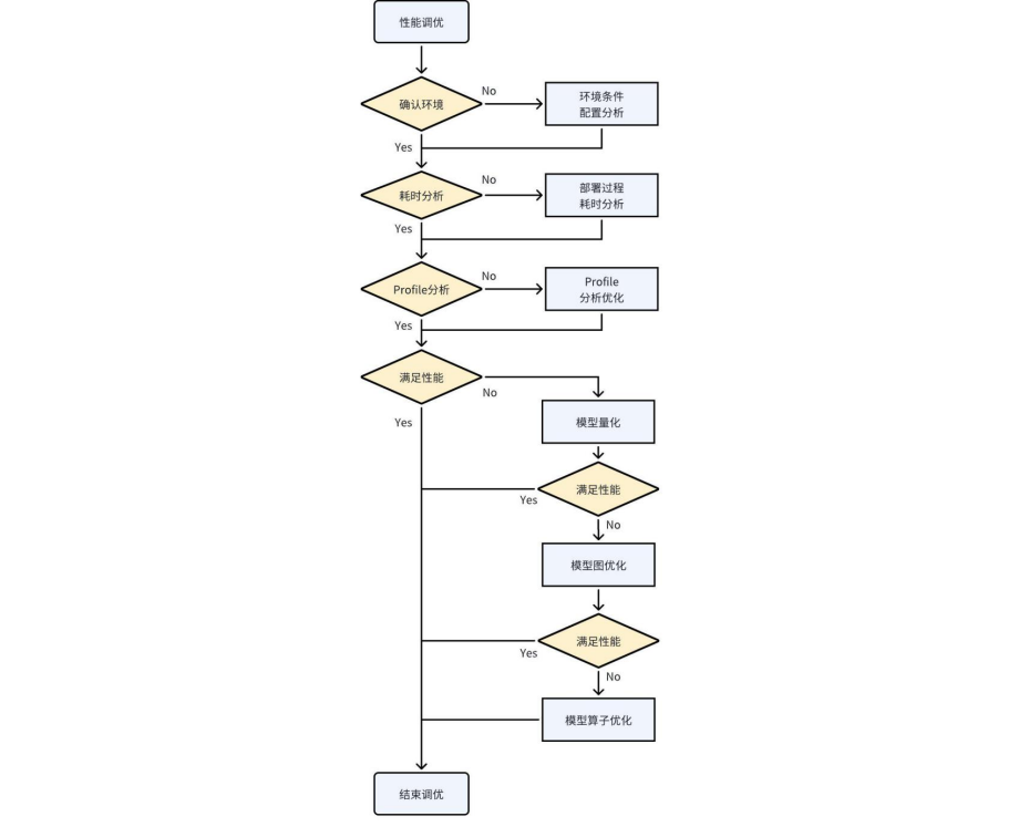
Figure 5-2 Model performance optimization flow
5.2.1 Process of Model Performance Optimization Analysis
5.2.1.1 CHECKING THE RUNTIME ENVIRONMENT
At the beginning of all performance analysis and optimization, the baseline of the test environment should be established first. Only when the baselines are the same is the measured performance data meaningful. For example, the inference performance of the same model tested without fixed frequencies fluctuates considerably, so the time consumption of a batch of tests cannot be taken as the average single-frame time.
There are several aspects to consider when querying and setting the conditions and configuration of the test environment:
Querying and setting the CPU, DDR, and NPU frequencies
The fixed frequency directly affects the execution speed; the higher the frequency, the relatively better the performance. The relationship between frequency changes and performance improvement is not linear. Increasing the frequency relatively increases power consumption as well. Refer to the following link for fixed frequency commands: https://github.com/airockchip/rknn_model_zoo/blob/main/scaling_frequency.sh
Alternatively, you can simply use the following command to set the performance mode:
echo performance | tee $(find /sys/ -name *governor) /dev/null || true
- Checking the NPU kernel driver version
The performance optimization items of some features or operators are related to the kernel driver version, and newer kernel driver versions can apply the latest underlying optimization implementations. Therefore, please check whether a relatively recent kernel driver version is in use. Currently, it is recommended to update to a version later than 0.9.2. This step is not a mandatory update.
The commands for checking the kernel driver version are as follows:
cat /sys/kernel/debug/rknpu/version # for RK3566/RK3568/RK3588/RK3562/RK3576
cat /proc/rknpu/version # for RV1106 series/RV1103 series/RV1126B
- Checking the NPU load
The NPU load is the percentage of time the NPU spends executing tasks within a unit of time. The load reflects how busy the NPU is. If the queried load is low, it indicates that the NPU is waiting for task submissions for a longer time, and it is necessary to check the time consumed by data input/output copies, the optimization of pre-processing and post- processing in the application, and so on. Alternatively, use a multi-threaded processing approach in the application to increase the NPU load.
Also note that the NPU load does not represent the actual MAC utilization. MAC utilization reflects the execution efficiency of the running tasks in the NPU hardware units.
The commands for querying the NPU load are as follows:
cat /sys/kernel/debug/rknpu/load
# or
cat /proc/debug/rknpu/load
5.2.1.2 DEPLOYMENT TIME ANALYSIS
The entire deployment process can be divided into three aspects in terms of time consumption: user application time, input-output data copy time, and model inference time. Analyzing the time distribution of each step can help identify optimization priorities. The time consumption of these steps can be measured by timestamping in the application.
User application time:
User application time mainly refers to the non-NPU-related time during the inference process. Typically, it includes pre-processing, post-processing, and the execution time of logical code. Users have full control over this part. If the application time is significantly high in proportion to the overall time, besides optimizing and simplifying the code, user can try to accelerate some operations using dedicated hardware.
For example, matrix multiplication and addition operations can be accelerated by using the Matmul API to invoke NPU-assisted computation. Similarly, image scaling operations can be accelerated by invoking the interfaces of RGA.
Input-output copy time:
When using the general API, there is a copy time involved between the input/output memory and the NPU memory. This time can be printed when calling the general API. The copy time depends on the performance of DDR and CPU. When the input-output data is small, the copy time is low. However, when the data is large, it’s time can’t be ignored. Therefore, it is recommended to use zero-copy APIs.
When using zero-copy APIs, the input-output memory is directly accessed by the NPU. For detailed usage of zero-copy interfaces, please refer to RKNN Runtime Zero-Copy Interface.
Inference time:
The time consumed by the NPU for inference is influenced by factors such as the size of the model and the version of the compiler optimization. The reasoning time of RKNN’s LOG printing is different at different RKNN_LOG_LEVEL levels because LOG printing takes a certain amount of time.
Generally, when viewing the time taken for single-frame inference, the LOG level is set to 1, and the average is taken after running multiple times.
5.2.2 Performance Analysis
5.2.2.1 OBTAIN PROFILE INFORMATION
When you need to know the layer-by-layer time consumption of model inference, you can enter the following command before running the program to print detailed information:
export RKNN_LOG_LEVEL=4
./run_rknn_test ./test.rknn ./input.jpg
If it is on the Android platform, you can obtain detailed logs through the logcat command after running.
If you are using rknn-toolkit2, you can use the following method to get the time consumption of each layer:
rknn.init_runtime(target=platform, perf_debug=True)
rknn.eval_perf()
The performance analysis report information is as follows (only the performance-related parts are excerpted)
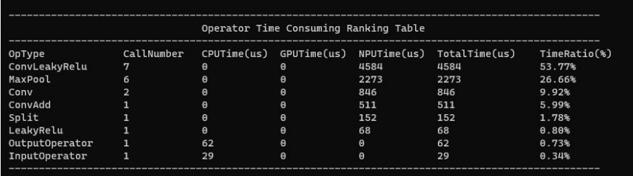
Figure 5-3 Performance analysis report
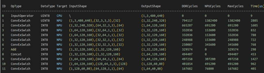
Figure 5-4 Performance analysis report
You can quickly locate the desired information from the overall performance profile and the layer- by-layer performance profile, and formulate subsequent optimization strategies with different focuses based on the data. After obtaining the profile, you can perform the following analyses: analyze the layer-by-layer time consumption to find the highly time-consuming operators; analyze the impact of non-NPU operators; analyze the performance bottlenecks of NPU operators. These are discussed in detail below.
5.2.2.2 ANALYZING THE TIME-CONSUMING LAYER BY LAYER
As shown in the figure below, you can find the highly time-consuming operators from the Time column and optimize them first. You can also look at the Op Type column to find out whether the highly time-consuming operators belong to the same OpType, so that they can be optimized uniformly.
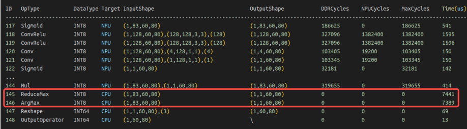
Figure 5-5 Performance analysis of highly time-consuming operators
It is worth noting that a highly time-consuming operator is not necessarily an inefficient operator. Some operators consume a large amount of computing power. When the MAC utilization of a highly time-consuming operator is very high, you should consider whether the size/scale of this operator can be reduced to decrease the time consumption. However, when highly time- consuming operators with very low utilization appear, these operators are the focus of optimization.
5.2.2.3 ANALYZE THE IMPACT OF CPU OPERATORS
As shown in the figure below, you can see that some highly time-consuming operators run on the CPU. Converting these CPU operators to run on the NPU can greatly mitigate the impact of their high time consumption. Generally speaking, most of users’ performance optimization problems are solved after converting the CPU operators to NPU. Therefore, pay special attention to the time consumption of CPU operators.
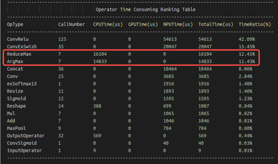
Figure 5-6 CPU operator performance analysis
Generally speaking, there are several reasons why an operator runs on a non-NPU:
The operator size exceeds the limit (check the operator size limit in the OpList document)
The operator does not yet support running on the NPU (check whether OpList supports this operator; you can submit an issue on the Github project)
NPU hardware limitations make it unsupported (check whether the algorithm can be equivalently replaced with another implementation supported by the NPU)
5.2.2.4 ANALYSIS OF NPU OPERATOR PERFORMANCE BOTTLENECKS
When considering the high time consumption of NPU operators, you can use the three columns DDR Cycles/NPU Cycles/Total Cycles to determine whether the theoretical bottleneck of the operator’s time consumption is a bandwidth bottleneck or a computing power bottleneck. The DDR Cycles here is data converted according to the NPU frequency, referring to the number of cycles required, at the NPU frequency, for the operator of that layer to read and write data, so it can be directly compared with the NPU Cycles.
As shown in the figure below:
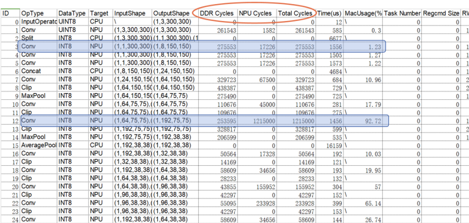
Figure 5-7 NPU operator performance bottleneck analysis
When the DDR Cycles of the third layer are much larger than the NPU Cycles, it means that the number of Cycles this layer spends reading and writing data is much greater than the number of Cycles required for the operation, so the bottleneck of this Conv comes from bandwidth.
When the DDR Cycles of the twelfth layer are much smaller than the NPU Cycles, it means that the number of Cycles this layer spends reading and writing data is much less than the number of Cycles required for the operation, so the bottleneck of this Conv comes from computing power.
Currently, the NPU Cycles column mainly displays the Cycles required by Conv; other operator types will be gradually added later.
5.2.3 Quantitative acceleration
Quantization can significantly reduce the calculation amount of the model and save bandwidth consumption. On the other hand, the INT8 computing power of NPU is much greater than that of FP16, so quantization can greatly improve the model running speed. We recommend using quantitative model deployment. For details on how to use model quantification, see Introduction to Quantization.
5.2.4 Graph optimization
Graph optimization of the model is the easiest way to coordinate and optimize the model from an overall perspective. After analyzing the operators or subgraphs that take a high proportion of time, we can transform the graph in many different ways to achieve optimization. Graph optimization mainly aims at saving redundant operators, converting non-NPU OPs into NPUs, and transforming hardware-oriented high-efficiency operators. These goals may sometimes be contradictory. For example, in order to convert non-NPU OP to NPU, a few additional operators may be needed. This may seem to violate the goal of saving redundant operators, but the overall inference performance improvement is beneficial. meaningful.
In the RKNN-Toolkit2 toolchain, the software stack already performs graph optimization to a certain extent during the model conversion process. However, this process is not omnipotent and perfect. Some scenarios that have not been considered will still have redundant operations. Users can perform pre-emptive graph optimization based on some of the ideas introduced in this section. The following is only an introduction to each optimization method. It is not mandatory and needs to be used flexibly in actual scenarios.
5.2.4.1 CONVERT NON-NPU OP TO NPU OP
For non-NPU ops, some equivalent graph transformations can be made to replace them with operators supported by the NPU, so as to achieve the optimization purpose of converting them to NPU.
For example, in the figure below, taking the shufflenetv2_0.5 model as an example, the channel shuffle operation in it is replaced with an approximate convolution. The weight values are 0/1, which can achieve the effect of rearranging data. If the Transpose and Reshape operations cannot be implemented on the NPU, these operators can be consolidated into a Conv operator to achieve the data rearrangement.
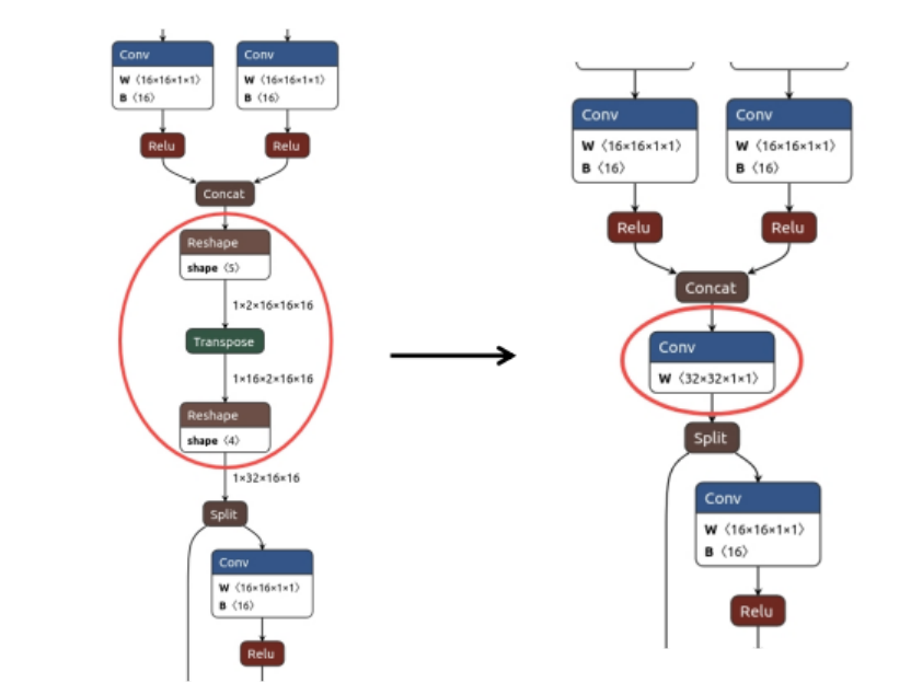
Figure 5-8 Convolution rearrangement
5.2.4.2 USE HARDWARE FUSE FEATURE TO DESIGN NETWORK OR GRAPH OPTIMIZATION
The NPU supports fusing some operator combinations. The operation flow of some operators can be appropriately adjusted to adapt to the NPU fusion rules and achieve operator fusion optimization.
Although the RKNN software stack performs a certain degree of graph optimization, it cannot fully cover all situations. In some special cases, there may be graph structures that could theoretically be fused and simplified, but that the final graph optimization fails to fuse. Users can manually adjust the algorithm to quickly solve this optimization problem.
For example, in the figure below, without changing the correctness of the calculation, by adjusting the order of the Transpose and Clip operators, Conv and Clip are fused in the operation, improving performance.
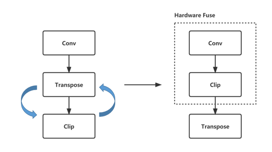
Figure 5-9 Operator graph optimization/fusion
Design with the fusion rules. The fusion rules are as follows:
| Supported fusion rules | Fusion rules supported by future plans |
|---|---|
| Conv+Relu | Activation+Add(Mul) |
| Conv+PRelu(LeakyRelu) | Add(Mul)+Activation |
| Conv+Clip | Conv+Mul |
| Conv+Sigmoid(Tanh/Elu/Silu…) | Conv+Activation+Mul |
| Conv+Add | Conv+Activation+Pooling |
| Conv+Activation+Add | Conv+Activation+Add(Mul)+Pooling |
5.2.4.3 SUBGRAPH TRANSFORMATION
When analyzing a certain graph region, the algorithm design for implementing a certain behavior sometimes pursues clarity of expression without considering the performance impact on the actual deployment, which easily produces complex and redundant graph structures. Through algorithmic equivalence, the subgraph of a certain region can be converted into a single OP, reducing the operator calculation steps and achieving the optimization purpose.
For example, the figure below shows the equivalent graph transformation of Yolov5-nano, which consolidates several complex Slice data extractions into a Conv, forming a new Conv and greatly simplifying the graph structure.
Solution source: https://github.com/ultralytics/yolov5/issues/4825
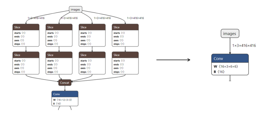
Figure 5-10 Operator equivalent graph transformation
5.2.4.4 “COMBINING SIMILAR TERMS” AND “EXTRACTING COMMON FACTORS”
When certain operators are computed multiple times in succession, they can be simplified and merged into the same operator, such as Reshape, Transpose, Slice, some Add/Mul/Sub/Div, etc.
For example, in the figure below, similar operators can be merged by simply adjusting the order of the graph.
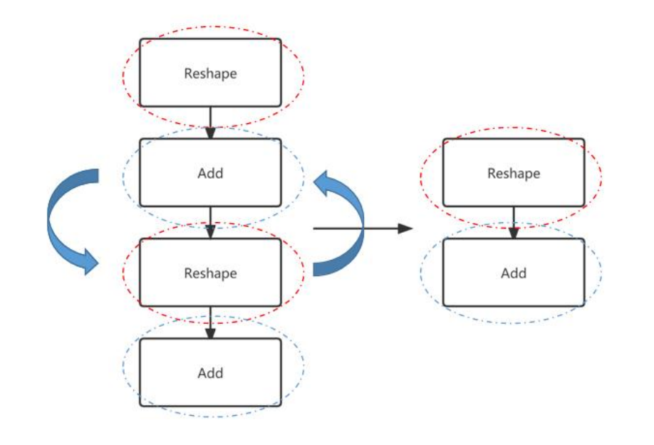
Figure 5-11 Operator merging of similar terms
Some graph structures have common parts with same-type operations that can be reordered and extracted into a single operation.
For example, in the figure below, by adjusting the operator order, the repetitive operators of the same type can be extracted separately so that the operation is executed only once.
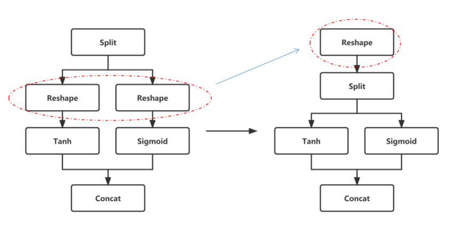
Figure 5-12 Repetitive operator merging
5.2.5 Operator level optimization
Operator-level optimization of a model is a highly targeted fine-grained optimization, involving the specific transformation design of certain operators to further improve performance. Operator optimization is mostly about targeted operator size design, so that operators run at the size specifications with the highest hardware implementation efficiency. For example, for some operators of similar size and scale, the running time consumption of aligned and non-aligned operations may differ greatly. The reason for the difference is that the hardware requires additional redundant operations to guarantee correctness for some operators with non-aligned sizes. Therefore, the size design of operators can also have a great impact on model performance. Users can perform operator optimization in advance according to the following ideas.
5.2.5.1 DDR-FRIENDLY OP SIZE DESIGN (NOT MANDATORY)
Under some aligned sizes, in addition to higher NPU computing efficiency, reading and writing to the DDR is also more friendly. Under the same bandwidth conditions, more friendly reading and writing improves the bandwidth efficiency of the DDR, thereby achieving better performance. The following lists some size rules that are more friendly to DDR reading and writing. These rules are not mandatory.
Channel aligned to the alignment amount
The alignment tables are shown below:
Table 5-1 RK3566/RK3568
| Conv | Depthwise Conv | Other OP | ||
|---|---|---|---|---|
| Dtype | Input Channel | Output Channel | Input & Output Channel | Input & Output Channel |
| Int8 | 32 | 16 | 32 | 8 |
| Int16 | 16 | 8 | 16 | 4 |
| Conv | Depthwise Conv | Other OP | ||
|---|---|---|---|---|
| Float16 | 16 | 8 | 16 | 4 |
| BFloat16 | 16 | 8 | 16 | 4 |
Table 5-2 RK3588/RK3576/RV1126B
| Conv | Depthwise Conv | Other OP | ||
|---|---|---|---|---|
| Dtype | Input Channel | Output Channel | Input & Output Channel | Input & Output Channel |
| Int8 | 32 | 32 | 64 | 16 |
| Int16 | 32 | 16 | 32 | 8 |
| Float16 | 32 | 16 | 32 | 8 |
| BFloat16 | 32 | 16 | 32 | 8 |
| TFloat32 | 16 | 16 | 16 | 4 |
Table 5-3 RV1106/RV1103
| Conv | Depthwise Conv | Other OP | ||
|---|---|---|---|---|
| Dtype | Input Channel | Output Channel | Input & Output Channel | Input & Output Channel |
| Int8 | 32 | 16 | 32 | 16 |
| Int16 | 16 | 16 | 16 | 8 |
Table 5-4 RK3562
| Conv | Depthwise Conv | Other OP | ||
|---|---|---|---|---|
| Dtype | Input Channel | Output Channel | Input & Output Channel | Input & Output Channel |
| Int8 | 32 | 16 | 32 | 16 |
| Int16 | 32 | 8 | 16 | 8 |
| Float16 | 32 | 8 | 16 | 8 |
| BFloat16 | 32 | 8 | 16 | 8 |
| TFloat32 | 16 | 8 | 8 | 4 |
4 aligned when Height * Width > 1
For operators of the same scale, a size with a larger Width and a smaller Height is more friendly to DDR reading and writing. As shown in the figure below, the convolution efficiency of the right figure is higher than that of the left figure
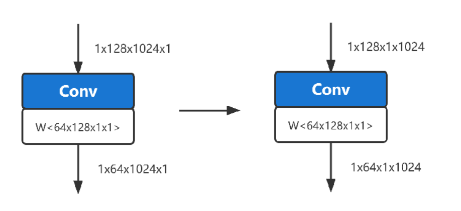
Figure 5-13 Comparison of convolutions of the same specification
5.2.5.2 DESIGN OF HIGH-UTILIZATION OPERATOR
In order to improve the overall utilization of computing power in model design, it is generally necessary to avoid inefficient operators and select operator size designs that are easy to achieve higher utilization. In the following chapters, we will list some inefficient operators that can be avoided as much as possible and discuss the relationship between convolution size and utilization.
Avoid inefficient operators
Try to reduce the following three types of operators in the model
Table 5-5 Three types of inefficient operators
| Data transfer | Size transformation | Non-Relu activation function |
|---|---|---|
| Transpose | Resize | Sigmoid |
| Reshape | Tile | Tanh |
| Split | Pooling | Softplus |
| Concat | Pad | Hardswish |
Relationship between convolution size and utilization
Since the performance of convolution will be affected by both computing power and bandwidth, MAC utilization is often used to illustrate the extent of hardware computing power when evaluating performance.
The relationship between convolution size and utilization is discussed here as a performance reference aid for users to design models. The following is a rough reference based on empirical data:
Notes on the following nouns: KH (kernel height), KW (kernel width), KC (kernel channel), type_bytes (weight bit width divided by 8), Ksize (KW or KH), Kstride (stride in the KW or KH direction)
When the channel of the convolutional input and output Tensor meets the alignment requirements (see aligning table data in 8.4.1), the utilization rate is higher.
When the channel of the input Tensor is < 256, the utilization rate is relatively high. When the channel is > 512, the utilization rate will gradually decrease as the channel increases.
In terms of weight size, the utilization rate is relatively high when KH* KW * KC * type_bytes < 6K Bytes. Utilization will drop significantly when it exceeds a certain size.
The larger the ratio of Ksize / Kstride, the higher the utilization rate. For example (Ksize=3, Kstride=1 is better than Ksize=2, Kstride=1)
The utilization rate decreases when the Height * Width of the output Tensor < 16.
The larger the Channel of the output Tensor, the higher the utilization rate.
The above discussion only examines the factors that affect utilization due to independent size. The actual MAC utilization shown by convolution in the actual deployment model is the result of a combination of many factors.
5.2.5.3 SUBGRAPH FUSION
The RKNN software stack will match certain specific graph relationships into custom operators, as shown in the figure below. If they are not fused into the corresponding operators, you can check whether the connection relationships are different, resulting in no match.
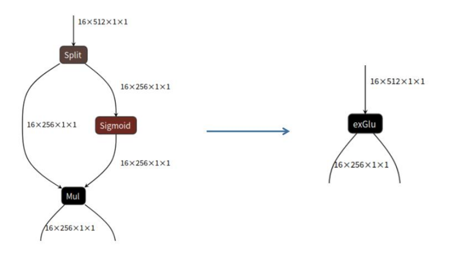
Figure 5-14 Glu subgraph fusion
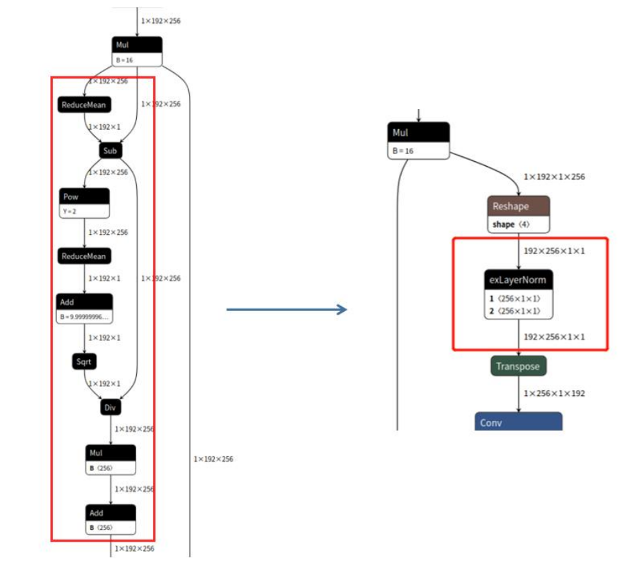
Figure 5-15 LayerNorm subgraph fusion
The currently supported subgraph fusion rules are:
Split + Sigmoid + Mul -> GLU
ReduceMean + Sub + Pow + ReduceMean + Add + Sqrt + Div (+ Mul + Add) -> LayerNorm