
ArmSoM applicability and source
This is a Rockchip platform reference, not an ArmSoM hardware test. The source is RKNN SDK User Guide V2.3.2, Chinese 165 pages and English 178 pages. Chinese follows the Chinese source; English, Russian and German follow the English source. Chinese original figures are used only in Chinese; all other versions use the English originals. The supported SoCs and software requirements in the source are retained below; support for a specific ArmSoM board, SDK/BSP, kernel driver and RKNN Runtime combination has not been verified. Confirm the board SoC, NPU driver, SDK/Runtime versions and supported operators before deployment. All performance, accuracy, memory, address and log examples originate from the source; no code was executed and no hardware was tested.
Same-version sources are not identical: the Chinese performance-analysis flowchart is absent from English; the English sparse-inference text adds a weight-channel limit greater than 32; the memory-evaluation example differs. Source typos, inconsistent API descriptions, missing values and clipped screenshot text are retained and documented, not silently corrected. Equations are provided as editable notation alongside source crops; round denotes the source rounding operation. See the editorial notes for page-specific details.
EDITORIAL-NOTES · ArmSoM · RKNN-Toolkit2
1 Introduction to RKNN
1.1 Introduction to RKNN Toolchain
1.1.1 Overview of the RKNN Software Stack
The RKNN software stack enables users to quickly deploy AI models to Rockchip chips. The overall framework is as follows:
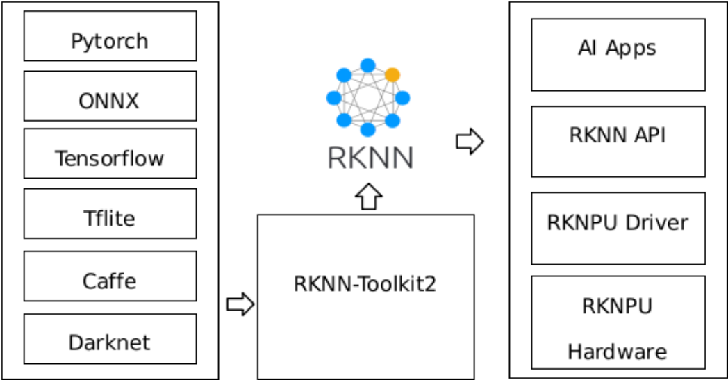
Figure 1-1 RKNN Software Stack
In order to use RKNPU, users need to first run the RKNN-Toolkit2 tool on the computer, convert the trained model into an RKNN format model, and then install it on the development board using the RKNN C API or Python.
1.1.2 Introduction to RKNN-Toolkit2 Features
RKNN-Toolkit2 is a development suite that allows users to convert, infer, and evaluate models on computer. The main diagram of RKNN-Toolkit2 is as follows:
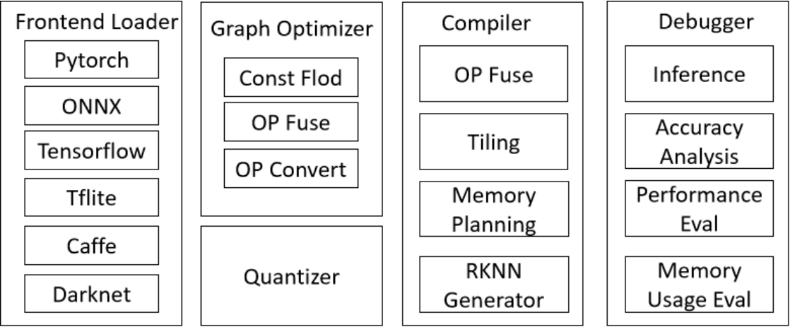
Figure 1-2 RKNN-Toolkit2 Software Diagram
The toolkit provides a convenient Python interface to perform the following functions:
1. Model Conversion: Support the conversion of PyTorch, ONNX, TensorFlow, TensorFlow Lite, Caffe, DarkNet, and other models into RKNN models.
2. Quantization Functionality: Support quantizing floating-point models into fixed-point models. It also supports mixed quantization functionality.
3. Model Inference: Distribute the RKNN model to the designated NPU device for inference and obtain the inference results; or simulate the NPU on the computer to run the RKNN model and obtain the inference results.
4. Performance and Memory Evaluation: Distributes the RKNN model to a designated NPU device to evaluate the performance and memory usage of the model when running on the actual device.
5. Quantization accuracy analysis: This function will give the cosine distance and Euclidean distance between the inference results of each layer of quantized model and that of floating-point model, so as to facilitate the analysis of how quantization errors occur and provide information for improving the accuracy of the quantization model.
6. Model Encryption: Encrypt the RKNN model as a whole using the specified encryption level.
1.1.3 Introduction to RKNN Runtime Features
RKNN Runtime is mainly responsible for loading the RKNN model and calling the NPU driver to infer the RKNN model on the NPU. When inferring the RKNN model, the original data must go through three major processes: input preprocessing, NPU running model, and output postprocessing. Currently, RKNN Runtime provides two processing flows, general API and zero-copy API, based on different model input formats and quantization methods.
General API: Provides a simple and straightforward set of inference APIs that are easy to use. The process is shown in Figure 1-3. Data normalization, quantization, data layout format conversion, and dequantization are performed on the CPU, while model inference is executed on the NPU.
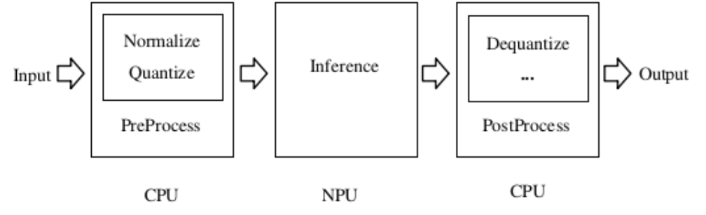
Figure 1-3 Data Processing Flow of the General API Zero-copy API: The process is shown in Figure 1-4. It optimizes the data processing flow of the general API. Data normalization, quantization, and model inference are all performed on the NPU, while the data layout conversion and dequantization of the NPU output are executed on the CPU or NPU. The zero-copy API has higher efficiency in handling the input data flow. It supports obtaining data between different IP cores without data copying to reduce CPU and DDR bandwidth consumption. For example, data obtained through a camera or decoded data can be directly imported into the NPU by zero-copy API.
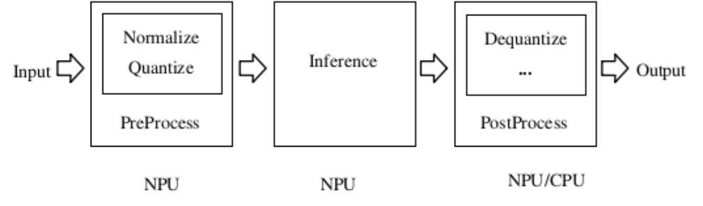
Figure 1-4 Data Processing Flow of the Zero-copy API
When the input data only has virtual address, only the general API can be used. When the input data has physical address or file descriptors (fd), both sets of API can be used.
1.2 Introduction to RKNN Development Process
Users can refer to the flowchart to understand the overall development steps of RKNN, which mainly include model conversion, model evaluation, and on-board deployment and execution.

Figure 1-5 RKNN Development Flowchart
1.2.1 Model Conversion
In this stage, the original deep learning model is converted into the RKNN format for efficient inference on RKNPU platforms. This step includes:
Obtaining the Original Model: Obtain or train a deep learning model using popular frameworks such as ONNX, PyTorch or TensorFlow.
Model Configuration: Fill in the necessary configuration parameters in RKNN-Toolkit2, such as mean values, normalization, quantization option, target platform, etc.
Model Loading: Import the model into RKNN-Toolkit2 using the appropriate loading interface and select the correct loading method according to the model type.
Model Building: Build the RKNN model using the rknn.build() interface. Users can choose whether to perform quantization to improve the model’s performance on the hardware.
Model Export: Export the RKNN model as a file (.rknn format) using the rknn.export_rknn() interface for future deployment.
For more detailed information, please refer to chapters 3.1 and 4.2.1.
1.2.2 Model Evaluation
The model evaluation stage helps users analyze model performance, quantization accuracy and memory usage on the board. The main steps of evaluation include the following operations:
PC-to-Board Model Debugging: This phase involves using Python to connect PC to the RKNPU platform for inference and model validation, which covers preprocessing of input data and post-processing of output results to ensure that the model runs correctly on the board.
Accuracy Evaluation: Use the rknn.accuracy_analysis() interface, comparing the output analysis of quantization errors between quantization models and floating-point models.
Performance Evaluation: Use rknn.eval_perf() interface to understand the inference performance of the model on the platform, helping users further optimize the model structure and speed up inference performance.
Memory Evaluation: Use the rknn.eval_memory() interface to understand the memory usage of the model on the board, helping users further optimize the model structure and minimize memory usage.
For more detailed information, please refer to chapters 3.2, 3.3, 4.2.2, and 4.2.3.
1.2.3 Board-side Deployment and Execution
This stage covers the actual deployment and execution of the model. It typically includes the following steps:
Model Initialization: Load the RKNN model into the RKNPU platform and prepare for preprocessing.
Model Preprocessing: Load the input data into the RKNPU platform and prepare for inference.
Model Inference: Perform the inference operation by passing the input data to the model and obtaining the inference results.
Model Postprocessing: Get the inference results for postprocessing and pass the postprocessed results to the application side.
Model Release: After completing the inference process, release the model resources for other tasks to use the RKNN model.
For more detailed information, please refer to chapters 3.4 and 4.2.3.
These three steps constitute the complete RKNN development process, ensuring the successful conversion, debugging, evaluation, and efficient deployment of artificial intelligence models on the RKNPU.
1.3 Supported Hardware Platforms
This document applies to the following hardware platforms:
RV1103, RV1103B, RV1106, RV1106B, RK2118, RK3562, RK3566 series, RK3568 series, RK3576, RK3588 series, RV1126B
Note: RK3566_RK3568 is used to indicate RK3566/RK3568 series in this document. RK3588 is used to indicate RK3588/RK3588S series in this document.
1.4 Glossary
RKNN Model: It is the binary file running on the RKNPU, with the suffix .rknn.
Inference with board: It refer to using RKNN-Toolkit2 API interface to run the model. Actually, the model is running on the NPU on the development board.
DRM: It is the Direct Rendering Manager, a main stream of graph displaying framework on linux.
tensor: A multi-dimensional array of data.
fd: It is the file descriptor for representing the buffer.
NATIVE_LAYOUT: It refers to the native layout of NPU. In other words, it has the best performance when NPU is processing data with this memory layout.
i8 model: A quantized RKNN model which running by 8-bit signed integer data.
fp16 model: A non-quantized RKNN model which runs with 16-bit half-float data.
2 Development Environment Setup
RKNN-Toolkit2 supports two different version, one is for the x86, another one is for the ARM64. Both has the same installation setup except for ARM64 has not supported docker yet. Besides, ARM64 only supports models from the onnx and pytorch framework for conversion. Models from other frameworks does not support at the moment.
The difference between the version of x86 and ARM64:
| Deepleanring Framework | x86 | ARM64 |
|---|---|---|
| Caffe | ✔ | ✗ |
| TensorFlow | ✔ | ✗ |
| TF Lite | ✔ | ✗ |
| ONNX | ✔ | ✔ |
| DarkNet | ✔ | ✗ |
| PyTorch | ✔ | ✔ |
The difference in tools:
| Dependent Tools | x86 | ARM64 |
|---|---|---|
| adb | ✔ | ✗ |
| rknn_server | ✔ | ✗ |
| rknn runtime | ✔ | ✔ |
The difference when using x86 or ARM64:
The major difference is on using debugging function, such as accuracy analysis or inference, ARM64 is installed on ARM64 Linux, then using these functions mentioned above, only need to ensure that the librknnrt.so is located on ‘/usr/lib64’. Since the ARM64 does not support adb, it only works on current board. But x86 requires updating and utilizing the rknn_server and ensure that adb is available for using these debugging functions and connecting to other board if required.
Apart from that, x86 and ARM64 might have performance difference when it comes to accuracy analysis or quantizing.
Note: For RK2118 development environment preparation, please refer to “Rockchip_RK2118_Quick_Start_RKNN_SDK_EN”.
2.1 Installation of RKNN-Toolkit2
This chapter provides two methods for installing RKNN-Toolkit2: Docker and Pip. Users can choose either method according to their preferences.
2.1.1 Installation via Docker
2.1.1.1 Install Docker
Users who have already installed Docker can skip this step. For users who haven’t installed Docker, please follow the official manual for installation. Official Docker installation manual link: https://docs.docker.com/install/linux/ docker-ce/ubuntu/.
Note: Make sure to add the user to the docker group.
# Create docker group
sudo groupadd docker
# Add the current user to the docker group
sudo usermod -aG docker $USER
# Update and activate the docker group
newgrp docker
# Verify that sudo is not needed to execute docker commands
docker run hello-world
If it works, the results are as follows:
Unable to find image 'hello-world:latest' locally
latest: Pulling from library/hello-world
719385e32844: Pull complete
Digest: sha256:88ec0acaa3ec199d3b7eaf73588f4518c25f9d34f58ce9a0df68429c5af48e8d
Status: Downloaded newer image for hello-world:latest
Hello from Docker!
2.1.1.2 Image Preparation
This section introduces two methods for preparing the RKNN-Toolkit2 image environment, and users can choose either method.
1. Creating an Image Environment via Dockerfile
In the docker/docker_file folder of the RKNN-Toolkit2 project, the Dockerfile file for building the RKNN- Toolkit2 development environment is provided. Users can create the image using the following command:
cd docker/docker_file/ubuntu_xx_xx_cpxx
docker build -f Dockerfile_ubuntu_xx_xx_for_cpxx -t rknn-toolkit2:x.x.x-cpxx .
2. Load Pre-packaged Docker Image with all Development Environments
Download the corresponding version of the RKNN-Toolkit2 project file. After decompression, a Docker image that has packaged all development environments is provided in the docker/docker_image folder.
Network disk download link: https://console.zbox.filez.com/l/I00fc3. Extraction code: rknn.
Execute the following command to load the image file corresponding to the Python version:
docker load --input rknn-toolkit2-x.x.x-cpxx-docker.tar.gz
2.1.1.3 Querying Image Information
After the image is created or loaded successfully, check the Docker image information:
docker images
The relevant RKNN-Toolkit2 image information will be displayed:
REPOSITORY TAG IMAGE ID CREATED SIZE
rknn-toolkit2 x.x.x-cpxx xxxxxxxxxxxx 1 hours ago 5.89GB
2.1.1.4 Running the Image
Execute the following command to run the Docker image, users will enter the bash environment of the image.
docker run -t -i --privileged -v /dev/bus/usb:/dev/bus/usb rknn-toolkit2:x.x.x-cpxx /bin/bash
Users can map the “examples” folder code into the docker environment by appending the “-v <host src folder>: <image dst folder>” parameter.
docker run -t -i --privileged -v /dev/bus/usb:/dev/bus/usb -v /your/rknn-toolkit2-x.x.x/examples:/examples rknn-toolkit2:x.x.x-cpxx /bin/bash
2.1.1.5 Running the Demo
cd examples/onnx/yolov5
python test.py
After successfully running the script, the results should be as follows:
class score xmin, ymin, xmax, ymax
--------------------------------------------------
person 0.884 [ 208, 244, 286, 506]
person 0.868 [ 478, 236, 559, 528]
person 0.825 [ 110, 238, 230, 534]
person 0.339 [ 79, 353, 122, 516]
bus 0.705 [ 92, 128, 554, 467]
2.1.2 Installation via Pip
2.1.2.1 Install Python Environment
If the Python environment is already installed, users can skip this step.
sudo apt-get update
sudo apt-get install python3 python3-dev python3-pip
sudo apt-get install libxslt1-dev zlib1g zlib1g-dev libglib2.0-0 libsm6 libgl1-mesa-glx libprotobuf-dev gcc
If users want to install the RKNN-Toolkit2 in the local environment (non-Conda virtual environment), please proceed to step 2.1.2.4 after installing Python successfully.
2.1.2.2 Install Conda Tool
If there are multiple versions of Python installed on the system, it is recommended to use Conda to manage the Python environment.
Check whether Conda is installed and the version. If it is already installed, users can skip this step.
conda -V
# Prompt conda: command not found means conda is not installed.
# Successful installation will display the version such as: conda X.X.X
# X.X.X means version number, such as 23.9.0.
Download the Conda installation package:
wget -c https://github.com/conda-forge/miniforge/releases/latest/download/Miniforge3-Linux-x86_64.sh
Install Conda:
chmod 777 Miniforge3-Linux-x86_64.sh
bash Miniforge3-Linux-x86_64.sh
ARM64 version:
Download the Conda installation package:
wget -c https://github.com/conda-forge/miniforge/releases/latest/download/Miniforge3-Linux-aarch64.sh
Install Conda:
chmod 777 Miniforge3-Linux-aarch64.sh
bash Miniforge3-Linux-aarch64.sh
2.1.2.3 Create RKNN-Toolkit2 Conda Environment
Enter the Conda base environment:
source ~/miniforge3/bin/activate # Miniforge install directory path
# (base) xxx@xxx-pc:~$
Create a Conda environment named “RKNN-Toolkit2” with Python 3.8 version (recommand version):
conda create -n RKNN-Toolkit2 python=3.8
Enter the ‘RKNN-Toolkit2’ Conda environment:
conda activate RKNN-Toolkit2
# (RKNN-Toolkit2) xxx@xxx-pc:~$
2.1.2.4 Install RKNN-Toolkit2
After activating the ‘RKNN-Toolkit2’ Conda environment, you can install RKNN-Toolkit2 using either the pip source or a local wheel package:
Install via pip source
pip install rknn-toolkit2 -i https://pypi.org/simple

# If RKNN-Toolkit2 is already installed, you can upgrade it with the following command:
pip install rknn-toolkit2 -i https://pypi.org/simple --upgrade
Install via local wheel package
# Please choose the appropriate requirements file based on the Python version and processor architecture:
# where cpxx is the Python version
pip install -r /rknn-toolkit2/packages/x86_64/requirements_cpxx.txt
# pip install -r /rknn-toolkit2/packages/arm64/arm64_requirements_cpxx.txt

# Install RKNN-Toolkit2
# Please choose the appropriate wheel package file based on the Python version and processor architecture:
# where x.x.x is the RKNN-Toolkit2 version number, cpxx is the Python version
pip install /rknn-toolkit2/packages/x86_64/rknn_toolkit2-x.x.x-cpxx-cpxx-manylinux_2_17_x86_64.manylinux2014_x86_64.whl
# pip install /rknn-toolkit2/packages/arm64/rknn_toolkit2-x.x.x-cpxx-cpxx-manylinux_2_17_aarch64.manylinux2014_aarch64.whl
If no error occurs after executing the following command, the installation is successful.
$ python
>>> from rknn.api import RKNN
2.2 NPU Device Environment Setup
2.2.1 NPU Driver Version Confirmation
Query commands:
dmesg | grep -i rknpu
# or
cat /sys/kernel/debug/rknpu/version
# or
cat /sys/kernel/debug/rknpu/driver_version
# or
cat /proc/debug/rknpu/driver_version
Query results:
RKNPU driver: vX.X.X
X.X.X means version number such as 0.9.2.
Rockchip’s firmware comes with RKNPU driver pre-installed. If the above commands cannot query the NPU driver version, it may be that the third-party firmware has not installed the RKNPU driver. Open the kernel config file with the “CONFIG_ROCKCHIP_RKNPU=y” option, recompile the kernel driver and flash it. It is recommended that the RKNPU driver version is >= 0.9.2.
2.2.2 NPU Device Connection Environment Confirmation
The PC-to-board debugging function of RKNN-Toolkit2 requires the RKNN Server on the development side. It is a background proxy service running on the device, responsible for receiving commands and data transmitted from the computer via USB, executing the corresponding interfaces, and returning results to the computer. Therefore, it needs to be confirmed whether the device has started the RKNN Server.
Note: ARM64 does not need to use RKNN Server for debugging, skipping this step if you were using ARM64 for RKNN Toolkit2.
Check if there is an RKNN Server process running on the development board.
adb shell
ps | grep rknn_server
Query results:
702 root 1192 S grep rknn_server
If the RKNN Server process id is queried, it means RKNN Server starts normally. If the RKNN Server process id is not queried, execute the following command to manually start RKNN Server and then query.
Manually start RKNN Server on Android:
su
setenforce 0
nohup /vendor/bin/rknn_server >/dev/null&
RK356X/RK3576/RK3588/RV1126B Linux system to start RKNN Server manually:
nohup /usr/bin/rknn_server >/dev/null&
RV1103/RV1103B/RV1106/RV1106B Linux system to start RKNN Server manually:
nohup /oem/usr/bin/rknn_server >/dev/null&
Generally speaking, Rockchip’s firmwares integrate RKNN Server which starts automatically during boot-up. If there is no automatic startup or no relevant files for manual startup, please install or update RKNN Server manually.
2.2.3 RKNN Server Installation and Update
If the RKNN Server is not installed on the development board, the Runtime library is missing, or there is a version mismatch between the RKNN Server and the Runtime library, users will need to reinstall or update them. Here are two fundamental concepts:
1. RKNN Server: A background proxy service running on the development board. It receives data transmitted from the computer via USB, executes the corresponding interface of the board-side Runtime, and returns the results to the PC.
2. RKNPU2 Runtime Library
librknnrt.so: The Runtime library for RK3562/RK3566/RK3568/RK3576/RK3588/RV1126B development boards.
librknnmrt.so: The Runtime library for RV1103/RV1103B/RV1106/RV1106B development boards.
If RKNN Server is not installed on the board, the Runtime library does not exist, or the versions of RKNN Server and Runtime library are inconsistent, you need to reinstall or update.
Note:
1. If users are using an RKNN model with dynamic input dimensions, the RKNN Server and RKNPU2 Runtime library versions must be >= 1.5.0.
2. If you use a model larger than 2 GB, you must use the rknn_server version >=2.0.0b0.
3. On small memory platforms such as RV1103, RV1106, RV1103B and RV1106B, we recommend that you rknn_server version >=2.1.0.
4. It is important to ensure consistency among the versions of RKNN Server, Runtime library and RKNN- Toolkit2. It is recommended to install the latest versions of all components.
5. The rknn_server service on RK2118 is not used for board debugging with RKNN-Toolkit2. Instead, it facilitates the communication service between the DSP and the MCU.
6. ARM64 version does not require the RKNN Server. Thus, it does not need to update and utilize RKNN Server. But the debugging function depends on the RKNPU Runtime library and makes sure that it is latest verion on the board.
2.2.3.1 RK356X/RK3576/RK3588/RV1126B Platform
1. Android System
Check the versions of the RKNN Server and the librknnrt.so. If the version numbers are inconsistent, update them to the same version.
# Query rknn_server version
strings /vendor/bin/rknn_server | grep -i "rknn_server version"
# Display rknn_server version is X.X.X, such as 1.6.0
# rknn_server version: X.X.X
# Query the librknnrt.so library version

# 64-bit system
strings /vendor/lib64/librknnrt.so | grep -i "librknnrt version"
# 32-bit system
strings /vendor/lib/librknnrt.so | grep -i "librknnrt version"
# Display the librknnrt library version is X.X.X, such as 1.6.0
# librknnrt version: X.X.X
Update RKNN Server and librknnrt.so.
adb root
adb remount
64-bit system:
adb push runtime/Android/rknn_server/arm64/rknn_server /vendor/bin/
adb push runtime/Android/librknn_api/arm64-v8a/librknnrt.so /vendor/lib64
32-bit system:
adb push runtime/Android/rknn_server/arm/rknn_server /vendor/bin/
adb push runtime/Android/librknn_api/armeabi-v7a/librknnrt.so /vendor/lib
Restart the RKNN Server:
adb shell
su
chmod +x /vendor/bin/rknn_server
nohup /vendor/bin/rknn_server >/dev/null&
sync
reboot
2. Linux system
Check the versions of RKNN Server and the librknnrt.so. If the version numbers are inconsistent, update them to the same version.
# Check rknn_server version
strings /usr/bin/rknn_server | grep -i "rknn_server version"
# Display rknn_server version is X.X.X, such as 1.6.0
# rknn_server version: X.X.X

# Query the librknnrt.so version
strings /usr/lib/librknnrt.so | grep -i "librknnrt version"
# Display the librknnrt version is X.X.X, such as 1.6.0
# librknnrt version: X.X.X
Update RKNN Server and librknnrt.so.
64-bit system:
adb push runtime/Linux/rknn_server/aarch64/usr/bin/* /usr/bin
adb push runtime/Linux/librknn_api/aarch64/librknnrt.so /usr/lib64
32-bit system:
adb push runtime/Linux/rknn_server/armhf/usr/bin/* /usr/bin
adb push runtime/Linux/librknn_api/armhf/librknnrt.so /usr/lib
Restart the RKNN Server:
adb shell
chmod +x /usr/bin/rknn_server
nohup /usr/bin/rknn_server >/dev/null&
restart_rknn.sh
2.2.3.2 RV1103/RV1103B/RV1106/RV1106B Platform
Check the versions of the rknn_server and the librknnmrt.so. If the version numbers are inconsistent, update them to the same version.
# Query rknn_server version
strings /oem/usr/bin/rknn_server | grep -i "rknn_server version"
# Display rknn_server version is X.X.X, such as 1.6.0
# rknn_server version: X.X.X

# Query the librknnrt.so version
strings /oem/usr/lib/librknnmrt.so | grep -i "librknnmrt version"
# Display the librknnrt version is X.X.X, such as 1.6.0
# librknnmrt version: X.X.X
Update RKNN Server and librknnmrt.so. RV1103, RV1103B, RV1106 and RV1106B use the same RKNN Server and librknnmrt.so.
adb push runtime/Linux/rknn_server/armhf-uclibc/usr/bin/* /oem/usr/bin
adb push runtime/Linux/librknn_api/armhf-uclibc/librknnmrt.so /oem/usr/lib
Restart the RKNN Server:
adb shell
chmod +x /oem/usr/bin/rknn_server
nohup /oem/usr/bin/rknn_server >/dev/null&
restart_rknn.sh
2.2.4 View Detailed RKNN Server Logs
2.2.4.1 Android System
Enter the device terminal and set the log level:
adb shell
su
setenforce 0
setprop persist.vendor.rknn.server.log.level 5
Kill the current RKNN Server service process:
kill -9 `pgrep rknn_server`
If the RKNN Server does not restart automatically, users can start it manually and view detailed logs:
nohup /vendor/bin/rknn_server >/dev/null&
logcat
2.2.4.2 Linux System
Enter the device terminal and set the log level:
adb shell
export RKNN_SERVER_LOGLEVEL=5
Restart the RKNN Server to view detailed logs:
For the RK356X / RK3576 / RK3588 / RV1126B platform, run the following command:
nohup /usr/bin/rknn_server >/dev/null&
For the RV1103 / RV1103B / RV1106 / RV1106B platform, run the following commands:
nohup /oem/usr/bin/rknn_server >/dev/null&
3 RKNN Basic Instruction Guide
3.1 Model Conversion
RKNN-Toolkit2 provides many functions, including model conversion, performance analysis, deployment and debugging, etc. This section will focus on the model conversion function of RKNN-Toolkit2. Model conversion is one of the core functions of RKNN-Toolkit2, which allows users to convert various deep learning models from different frameworks to RKNN format running on RKNPU. Users can refer to the model conversion flow chart to help understand how to perform model conversion.
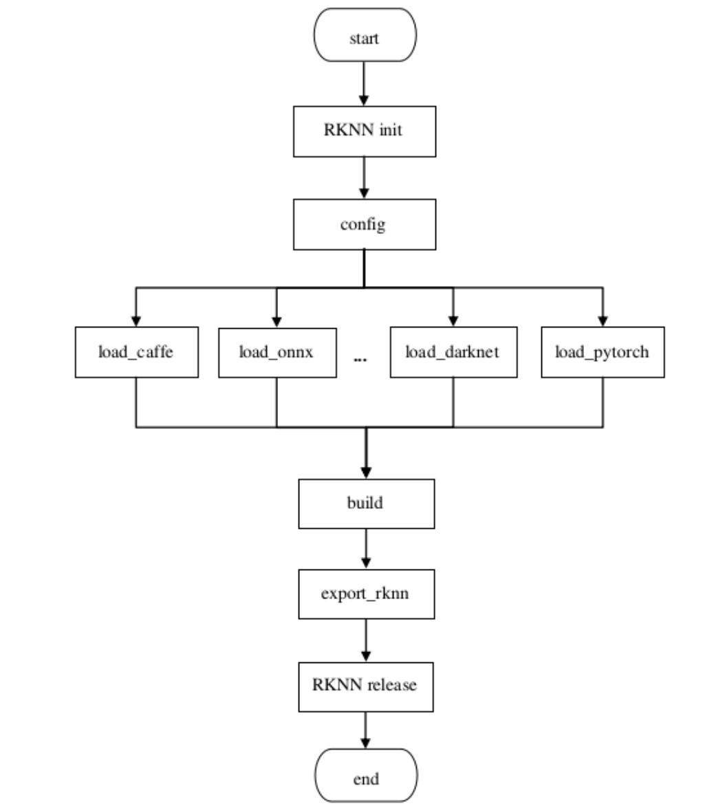
Figure 3-1 The flow chart of model conversion
Currently RKNN-Toolkit2 supports model conversion for multiple popular deep learning frameworks, including:
Caffe(recommended version is 1.0)
TensorFlow(recommended version is 1.12.0~2.8.0)
TensorFlow Lite(recommended version is Schema version = 3)
ONNX(recommended version is 1.7.0~1.10.0)
PyTorch(recommended version is 1.6.0~1.13.1)
Darknet(recommended version is Commit ID = 810d7f7)
Users can use the above framework to train or obtain pre-trained models and convert them into RKNN format for more efficient deployment and inference on the RKNPU platform.
3.1.1 RKNN Initialization and Release of object
In this part, users need to initialize the RKNN object first. This is the first step in the entire workflow.
Initialize the RKNN object:
Using the RKNN() constructor to initialize the RKNN object. Users can pass in the parameters verbose and verbose_file.
verbose determines whether to display detailed log information on the screen.
If the verbose_file parameter is set and verbose is set to True, log information will also be written to the specified file.
Example code:
rknn = RKNN(verbose=True, verbose_file='./mobilenet_build.log')
When all RKNN related operations are completed, the user needs to release resources. This is the last step of the entire workflow:
Release resources:
Using release() to release rknn object.
Example code:
rknn.release()
3.1.2 Config configuration explanation
Before model conversion, users need to set some configurations to ensure the correctness and performance of model conversion. Configuration parameters can be set through the rknn.config() interface, including setting the input mean, normalized value, whether to quantize, etc. Some commonly used configuration parameters are listed below:
mean_values and std_values are used to set the mean and normalized values of the input. These values are used in the quantification process, and the images no longer need to be averaged and normalized during the C API inferencing to reduce deployment time.
quant_img_RGB2BGR is used to control whether RGB to BGR conversion needs to be performed first when loading a quantization image during quantization. The default value is false. This configuration takes effect during quantification correction and will not take effect during the model inference stage. It needs to be processed by the users in pre-input processing. Please refer to Chapter 10.3 for detailed precautions. Note: Note: When quant_img_RGB2BGR= True, the model’s inference sequence is to perform RGB2BGR conversion first then perform mean_valuesand std_values operations later.
target_platform is used to specify the target platform of the RKNN model, supporting RV1103, RV1103B, RV1106, RV1106B, RV1126B, RK2118, RK3562, RK3566, RK3568, RK3576 and RK3588 at the moment.
quantized_algorithm is used to specify the quantization algorithm used when calculating the quantized parameters of each layer. You can choose normal, mmse or kl_divergence. The default algorithm is normal. For detailed description, see chapters 3.1.7, 6.1 and 6.2.
quantized_method supports layer or channel, used to determine whether the weights of each layer share parameters. The default is channel. For details, see chapters 3.1.7, 6.1 and 6.2.
optimization_level is used to modifying the model optimization level, you can turn off some or all of the optimization rules used in the model conversion process. The default value of this parameter is 3, which turns on all optimization options. When the value is 2 or 1, some optimization options that may affect the accuracy of some models are turned off. When the value is 0, all optimization options are turned off.
quantized_dtype is used to specify the quantization type. Currently, INT8 for linear asymmetric quantization is supported, and the default is ‘asymmetric_quantized-8’.
custom_string is used to adds custom string information to the RKNN model, such as version information of the model`s own iteration, etc. This information can be obtained by querying RKNN_QUERY_CUSTOM_STRING which facilitates special processing according to different RKNN models during deployment. The default value is None.
dynamic_input supports dynamic input and simulates the function of dynamic input according to multiple sets of input shapes specified by the users. The default value is None. See Chapter 5.4 for details.
For more specification of rknn.config(), please refer to the API manual. Only some common parameters are listed above.
Example code:
rknn.config(
    mean_values=[[103.94, 116.78, 123.68]],
    std_values=[[58.82, 58.82, 58.82]],
    quant_img_RGB2BGR=False,
    target_platform='rk3566')
3.1.3 Introduction to interface of model loading
According to different types of models, users need to use the corresponding loading interface to load model files. RKNN-Toolkit2 provides different loading interfaces, including Caffe, TensorFlow, TensorFlow Lite, ONNX, PyTorch, etc. The following is a brief introduction to various types of model loading interfaces:
Caffe loading:
Using rknn.load_caffe() to load the Caffe model.
Need to provide the model file (.prototxt suffix) path and the weight file (.caffemodel suffix) path.
If the model has multiple input layers, you can specify the order of the input layer names.
Example code:
ret = rknn.load_caffe(model='./mobilenet_v2.prototxt', blobs='./mobilenet_v2.caffemodel')
TensorFlow loading:
Using rknn.load_tensorflow() to load the TensorFlow model.
Need to provide the TensorFlow model file (.pb suffix) path, input node name, input node shape, and output node name.
Example code:
ret = rknn.load_tensorflow(tf_pb='./ssd_mobilenet_v1_coco_2017_11_17.pb',
              inputs=['Preprocessor/sub'],
              outputs=['concat', 'concat_1'],
              input_size_list=[[1, 300, 300, 3]])
TensorFlow Lite loading:
Usingrknn.load_tflite() to load the TensorFlow Lite model.
Need to provide the TensorFlow model file (.tflite suffix) path.
Example code:
ret = rknn.load_tflite(model='./mobilenet_v1.tflite')
ONNX loading:
Usingrknn.load_onnx() to load the ONNX model.
Need to provide the ONNX model file (.onnx suffix) path.
Example code:
ret = rknn.load_tflite(model='./mobilenet_v1.tflite')
DarkNet loading:
Usingrknn.load_darknet() to load the DarkNet model.
Need to provide the path to the DarkNet model file (.cfg suffix) and the weight file (.weights suffix).
Example code:
ret = rknn.load_darknet(model='./yolov3-tiny.cfg', weight='./yolov3.weights')
PyTorch loading:
Usingrknn.load_pytorch() to load the PyTorch model.
Need to provide the path to the PyTorch model file (.pt suffix), and the model must be in torchscript format.
Example code:
ret = rknn.load_pytorch(model='./resnet18.pt', input_size_list=[[1, 3, 224, 224]])
Users can select appropriate interfaces to load according to different types of models to ensure the model can be converted.
3.1.4 Construct RKNN Model
After the user loads the original model, the next is to build the RKNN model through the rknn.build() interface. When building a model, users can choose whether to perform quantization, which helps reduce the size of the model and improve performance on RKNPU. The rknn.build() interface parameters are as follows:
do_quantization controls whether to quantize the model, and it is recommended to set it to True.
dataset is used to provide the dataset used for quantitative calibration. The format of the dataset is a text file.
Example of dataset.txt :
./imgs/ILSVRC2012_val_00000665.JPEG
./imgs/ILSVRC2012_val_00001123.JPEG
./imgs/ILSVRC2012_val_00001129.JPEG
./imgs/ILSVRC2012_val_00001284.JPEG
./imgs/ILSVRC2012_val_00003026.JPEG
./imgs/ILSVRC2012_val_00005276.JPEG
Example code
ret = rknn.build(do_quantization=True, dataset='./dataset.txt')
3.1.5 Export RKNN Model
After building the RKNN model through the rknn.build() interface, the RKNN model can be saved as a file (.rknn suffix) through the rknn.export_rknn() interface for deployment. The interface parameters of rknn.export_rknn() are as follows:
export_pathThis the path to exported model file.
cpp_gen_cfgcan optionally generate C++ deployment examples.
Example code
ret = rknn.export_rknn(export_path='./mobilenet_v1.rknn')
These operations and interfaces cover the RKNN-Toolkit2 model conversion steps. According to different requirements and application scenarios, users can choose different configuration options and quantization algorithms for customized settings to facilitate subsequent deployment.
3.1.6 Model conversion tool: RKNN_Convert
RKNN_CONVERT is a model conversion tool provided by RKNN-Toolkit2. By encapsulating the above API interface, users only need to edit the yml configuration file corresponding to the model to convert the model through instructions. The following is an example command of how to use the rknn_convert tool and the supported command parameters:
python -m rknn.api.rknn_convert -t rk3588 -i ./model_config.yml -o ./output_path
By using the above commands and parameters, users can convert the model to RKNN format and save the converted model to the specified output path. The supported command parameters are described as follows:
-i: The path of model configuration file (.yml).
-o: The output directory of converted model.
-t: target_platform, the target platform can be rv1103, rv1103b, rv1106, rv1106b, rv1126b, rk2118, rk3562, rk3566, rk3568, rk3576 or rk3588.
-e: (Optional) Evaluate the model running time and memory usage of the model when running on the board. Please enter -e if it is enabled. Note: Be sure to connect the board and set the target_platform correctly, otherwise an error will be reported. When using multiple devices, the user should set -d device_id to select the device id.
-a: (Optional) Evaluate the accuracy of the generated rknn model. To enable the simulator accuracy evaluation, please enter on command line with -a “xx1.jpg xx2.jpg”. If users want to use accuracy analysis, please use it with the -d parameter.
-v: (Optional) Specify whether to print detailed log information on the screen. To enable printing mode, users need to enter -v on command line.
-d: (Optional) Using -d for a single adb device, -d device_id for multiple adb devices, and query device_id through adb devices.
The code shown below is an example of configuration for yaml:
models:
  # model output name
  name: object_detection
  # Original model framework
  platform: onnx
  # Model input file path
  model_file_path: ./object_detection.onnx
  # Describe information such as input and output shapes
  subgraphs:
   # model input tensor shape
   input_size_list:
    - 1,3,512,512
   # input tensor name
   inputs:
    - data
   # output tensor name
   outputs:
    - conv6-1
    - conv6-2
    - conv6-3
  # quantification flag
  quantize: true
  # Quantify dataset file path (relative yml path)
  dataset: ./dataset.txt
  configs:
   quantized_dtype: asymmetric_quantized-8
   # rknn.config mean_values
   mean_values: [127.5,127.5,127.5]
   # rknn.config std_values
   std_values: [128.0,128.0,128.0]
   # rknn.config quant_img_RGB2BGR
   quant_img_RGB2BGR: false
   # rknn.config quantized_algorithm
   quantized_algorithm: normal
This configuration file includes detailed information such as the name of the model, the framework used by the original model, the model file path, input and output information, and whether to perform quantification. Users can modify the corresponding configuration files according to the specific needs of the model.
The file appendix for yml configuration is shown below:
Table 3-1 yml parameter description of model conversion configuration
| Parameter | Content required to fill in |
|---|---|
| -name | Model output file name |
| -platform | The framework used by the original model, supporting tensorflow, tflite, caffe, onnx, pytorch, darknet |
| -model_file_path | Original model file path, suitable for one single model file, for example: tensorflow, tflite, onnx, pytorch |
| -quantize | Whether to use quantization |
| -dataset | The path of dataset for quantization (only required relative path). If accuracy_analysis was turned on, this option is required |
| -prototxt_file_path | When using caffe model, the prototxt file of the model |
| -caffemodel_file_path | When using caffe model, the caffemodel file of the model |
| -darknet_cfg_path | When using darknet model, the cfg file of the model |
| -darknet_weights_path | When using darknet model, the weight file of the model |
| -subgraphs | This section is for describing input and output shape and other model related information. In general, this parameter and the accompanying sub-parameters are optional. These values can be filled with model default values except for specific frameworks |
| —-input_size_list (Subparameter) |
The shape of input tensor |
| —-inputs (Subparameter) |
The name of input tensor |
| —-outputs (Subparameter) |
The output name of tensor |
| -configs | The corresponding rknn.config() configuration |
| —-quantized_dtype (Subparameter) |
Quantization type for RKNN-Toolkit2: User can fill in [asymmetric_quantized- 8]. If not entered, use the default value |
| —-mean_values (Subparameter) |
The mean of model input, e.g., the single model input is RGB, such as [123.675,116.28,103.53], if it was a model with multiple input, e.g., [[123,116,103],[255,255,255]] |
| —-std_values (Subparameter) |
The std of model input. For example, the model is a single input RGB, such as [58.395,58.295,58.391], and the model is a multiple input such as [[127,127,127], [255,255,255]] |
| —- quant_img_RGB2BGR (Subparameter) |
It denotes whether users need to do RGB2BGR when loading images for quantization. The default value is false |
| —-quantized_algorithm (Subparameter) |
Quantization algorithm, option including [‘normal’, ‘kl_divergence’, ‘mmse’], default value is normal |
| —-quantized_method (Subparameter) |
Quantization method, RKNN_toolkit2 option including [‘layer’, ‘channel’], using channel by default |
| —-optimization_level (Subparameter) |
Set optimization level. The default value is 3, using all default optimization options |
| —-model_pruning (Subparameter) |
Prune the model to reduce model size, defaults to false, turns on to true |
| —-quantize_weight (Subparameter) |
When the quantize parameter is false, the size of the rknn model is reduced by quantizing some weights. Default is false, enable is true |
| —-single_core_mode (Subparameter) |
Whether to generate only single-core models can reduce the size and memory consumption of RKNN models. The default value is false. Currently only valid for RK3576/RK3588. The default value is false. |
3.1.7 Model Quantization Function of RKNN-Toolkit2
RKNN-Toolkit2 provides two quantization methods and three quantization algorithms, which users can choose through the quantized_algorithm and quantized_method parameters in rknn.config(). The following is an introduction to these quantization algorithms and feature quantification methods:
Three quantization algorithms:
1. Normal quantization algorithm: Determining the maximum and minimum values of the quantization range by calculating the maximum and minimum floating point values of the features in the model. The algorithm is characterized by fast speed, but the effect is poor when the feature distribution is uneven. The recommended amount of quantified data is generally about 20-100 data sample.
2. MMSE quantization algorithm: Determining the maximum and minimum values of the quantization range by minimizing the mean square error loss of floating-point numbers and quantized and de-quantized floating-point numbers, which can alleviate the problem of quantization accuracy loss caused by large outliers to a certain extent. Due to the violent iteration method, the speed is slower, but it usually has higher accuracy than normal. The recommended amount of quantified data is generally about 20-50 data sample. Users can also increase or decrease the amount of quantified data appropriately according to the length of quantization time.
3. KL-Divergence quantification algorithm: abstract the floating-point numbers and fixed-point numbers in the feature in the model into two distributions, update the distribution of floating-point numbers and fixed-point numbers by adjusting different thresholds, and measure the two according to KL divergence The similarity of distributions is used to determine the maximum and minimum values of the quantization range. The time taken will be longer than normal, but much less than mmse. In some scenarios (when the feature distribution is not ideal), better improvement results can be obtained. The recommended amount of quantified data is generally about 20-100 images.
Two quantification methods:
1. Layer quantization method: Layer quantization method quantizes all channels of the same layer network as a whole, and all channels share the same quantization parameters.
2. Channel quantization method: Channel quantization method quantizes each channel of the same layer network independently, and each channel has its own quantization parameters. Usually, the channel quantization method has higher accuracy than Layer quantization method.
Based on the actual model quantification effect and requirements, users can choose appropriate quantification algorithms and feature quantification methods. For more detailed quantification instructions and principles, please seeChapter 6.
3.2 Model Assessment
3.2.1 Model Inferencing
After the original model is converted into an RKNN model, model inference can be performed on the simulator or on the board, and the inference results can be post-processed to check whether they are correct. If the inference results are incorrect, you can use accuracy analysis on the quantitative model and check whether the pre- and post- processing processes are correct or not.
Initialize the rknn.init_runtime() interface parameters as follows:
target: target hardware platform. The default value is None, inference will run on the simulator. When users need to obtain the actual inference results of the board side, users need to fill in the corresponding platform (RV1103 / RV1103B / RV1106 / RV1106B / RV1126B / RK3562 / RK3566 / RK3568 / RK3576 / RK3588).
device_id: device number. The default is None. If target is set, only one device will be selected for inference. If the computer is connected to multiple devices for board inference, the corresponding device ID needs to be specified. If perform model inference on a device using ADB over the network, the user needs to manually execute the command “adb connect [IP]” to connect to the device, and then enter the device identifier, typically in the form of an IP address or IP address followed by a port number. Use the adb devices command to list all connected devices.
perf_debug: Whether to enable debug mode when performing performance evaluation. The default value is False, and the total running time of the model can be obtained by calling the rknn.eval_perf() interface. When set to True, users can additionally obtain the running time of each layer, which is not supported by RV1103, RV1103B , RV1106 and RV1106B platforms.
eval_mem: Whether to enter memory evaluation mode. The default value is false. After setting it to True to enter memory evaluation mode, users can call the rknn.eval_memory() interface to obtain the memory usage when the model is running.
rknn.inference() interface parameters are as follows:
inputs: List of inputs to be inferred, in ndarray format.
data_format: The layout list of input data, which is only valid for 4-dimensional inputs. The format can be “NCHW” or “NHWC”. The default value is None, which means all input layouts are NHWC.
Example code:
ret = rknn.init_runtime(target=platform, device_id='515e9b401c060c0b')

# Preprocess
image_src = cv2.imread(IMG_PATH)
img = preprocess(image_src)

# Inference
outputs = rknn.inference(inputs=[img])

# Postprocess
outputs = postprocess(outputs)
Note:
1.If users encounter the “E RKNN: failed to allocate fd, ret: -1, errno: 12” error when inferring on the RV1103 or RV1106 platform, users can excute script RkLunch-stop.sh in the board terminal to close other applications that occupy memory.
2.In ARM64 version, rknn.init_runtime() is not supported for device_id
3.2.2 Model Accuracy Analysis
If there are problems with the quantitative model inference results, you can use the rknn.accuracy_analysis() to analyse the accuracy and check the accuracy of each layer of operators.
Accuracy analysisrknn.accuracy_analysis()interface parameters are as follows:
inputs: a list of file input paths (formats include jpg, png, bmp, and npy).
output_dir: The saved directory, the default value is ‘./snapshot’.
Target: Target hardware platform. Default value is None. If the target (RV1103 / RV1103B / RV1106 / RV1106B / RV1126B / RK3562 / RK3566 / RK3568 / RK3576 / RK3588) is set, the results of each layer at runtime will be obtained and accuracy analysis will be performed.
device_id: Device ID. Default is None, only using the emulator for precision analysis. If the target is set, only one device will be selected for accuracy analysis. If the computer is connected to multiple devices, the corresponding device ID needs to be specified. If perform precision analysis on a device using ADB over the network, the user needs to manually execute the command “adb connect [IP]” to connect to the device, and then enter the device identifier, typically in the form of an IP address or IP address followed by a port number.
Note:
1. During precision analysis, the operation may fail because the model is too large and the storage capacity on the board is insufficient. Users can use the df -h command on the board terminal to confirm the storage capacity. If there is insufficient space, delete useless files to ensure that the corresponding partition of output_dir has enough space to save result files.
2. After loading the RKNN model through rknn.load_rknn(), the model accuracy analysis function can not be used because the RKNN model lacks the original model information.
3. In ARM64 version, rknn.accuracy_analysis() is not supported for device_id
Example code:
ret = rknn.accuracy_analysis(inputs=[img_path], target=platform, device_id='515e9b401c060c0b')
Accuracy analysis results shown below:
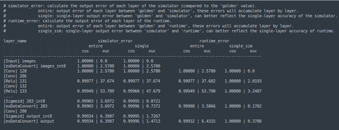
# simulator_error: calculate the output error of each layer of the simulator (compared to the 'golden' value).
# entire: output error of each layer between 'golden' and 'simulator', these errors will accumulate layer by layer.
# single: single-layer output error between 'golden' and 'simulator', can better reflect the single-layer accuracy of the simulator.
# runtime_error: calculate the output error of each layer of the runtime.
# entire: output error of each layer between 'golden' and 'runtime', these errors will accumulate layer by layer.
# single_sim: single-layer output error between 'simulator' and 'runtime', can better reflect the single-layer accuracy of runtime.
| layer_name | simulator_error entire cos | simulator_error entire euc | simulator_error single cos | simulator_error single euc | runtime_error entire cos | runtime_error entire euc | runtime_error single_sim cos | runtime_error single_sim euc |
|---|---|---|---|---|---|---|---|---|
| [Input] images | 1.00000 | 0.0 | 1.00000 | 0.0 | ||||
| [exDataConvert] images_int8 | 1.00000 | 2.5780 | 1.00000 | 2.5780 | ||||
| [Conv] 128 | 1.00000 | 2.5780 | 1.00000 | 2.5780 | 1.00000 | 2.5780 | 1.00000 | 0.0 |
| [Conv] 286 | ||||||||
| [Relu] 131 | 0.99977 | 37.674 | 0.99977 | 37.674 | 0.99977 | 37.682 | 1.00000 | 2.0193 |
| [Conv] 132 | ||||||||
| [Relu] 133 | 0.99949 | 53.789 | 0.99960 | 47.679 | 0.99949 | 53.790 | 1.00000 | 3.2487 |
| … | ||||||||
| [Sigmoid] 283_int8 | 0.99903 | 3.6972 | 0.99995 | 0.8721 | ||||
| [exDataConvert] 283 | 0.99903 | 3.6972 | 0.99996 | 0.7372 | 0.99908 | 3.5866 | 1.00000 | 0.1702 |
| [Conv] 280 | ||||||||
| [Sigmoid] output_int8 | 0.99934 | 6.3987 | 0.99995 | 1.7267 | ||||
| [exDataConvert] output | 0.99934 | 6.3987 | 0.99996 | 1.4713 | 0.99932 | 6.4315 | 1.00000 | 0.3788 |
Figure 3-2 Accuracy analysis results
It is divided into 4 columns of accuracy, as follows:
| simulator_error | entire | The cosine distance and Euclidean distance from the beginning to the current layer simulator result compared with the golden result. |
| single | When using the current layer golden input, the cosine distance and Euclidean distance are compared between the simulator result and the golden result. |
|
| runtime_error | entire | The cosine distance and Euclidean distance between the actual result and the golden result from the beginning to the end of the current layer. |
| single_sim | When the using current layer golden input, the cosine distance and Euclidean distance between the actual result of the current layer at the board end and the simulator result are compared. |
3.2.3 Model performance evaluation
The interface rknn.eval_perf() will output the current hardware frequency and obtain the performance evaluation results of the model. The fix_freq parameter indicates whether you need to try to fix the frequency of the hardware (including CPU/NPU/DDR). If you want to set the hardware frequency to True, otherwise Set to False, the default value is True. If the perf_debug parameter of rknn.init_runtime() is set to True during initialization, the time consumption of each layer and the total time consumption will be output. If it is False, only the total time consumption will be output.
Note:
1. Platform RV1103, RV1103B , RV1106 and RV1106B do not support perf_debug as True mode, and can only output the total time consumption of the model.
Example code:
ret = rknn.init_runtime(target=platform, perf_debug=True)
perf_detail = rknn.eval_perf()
Taking RK3588 as an example, the hardware frequency output after executing eval_perf is as follows (the frequencies supported by different firmware may vary). Among them, since the RK3588 CPU has a large and small core architecture, the CPU frequency column will output multiple frequency values in KHz. The NPU and DDR frequency units are both Hz.
CPU Current Frequency List:
  - 1800000
  - 2256000
  - 2304000
NPU Current Frequency List:
  - 1000000000
DDR Current Frequency List:
  - 2112000000
The result evaluation of performance is shown below:
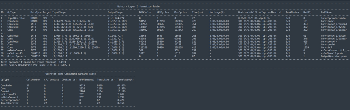
Network Layer Information Table
ID | OpType | DataType | Target | InputShape | OutputShape | DDRCycles | NPUCycles | MaxCycles | Time(us) | MacUsage(%) | WorkLoad(0/1/2)--ImproveTherical | TaskNumber | RW(KB) | FullName
1 | InputOperator | UINT8 | CPU | \ | (1,3,224,224) | 0 | 0 | 0 | 22 | \ | 0.0%/0.0%/0.0%--Up:0.0% | 0/0 | 0 | InputOperator:data
2 | ConvRelu | UINT8 | NPU | (1,3,224,224),(32,3,3,3),(32) | (1,32,112,112) | 94150 | 112896 | 112896 | 428 | 0.00/0.00/0.00 | 300.0%/0.0%/0.0%--Up:-200.0% | 3/0 | 151 | Conv:conv1
3 | ConvRelu | INT8 | NPU | (1,32,112,112),(32,32,1,1),(32) | (1,32,112,112) | 135965 | 50176 | 135965 | 351 | 0.00/0.00/0.00 | 300.0%/0.0%/0.0%--Up:-200.0% | 2/0 | 393 | Conv:conv2_1/expand
4 | ConvRelu | INT8 | NPU | (1,32,112,112),(1,32,3,3),(32) | (1,32,112,112) | 135884 | 112896 | 135884 | 383 | 0.00/0.00/0.00 | 300.0%/0.0%/0.0%--Up:-200.0% | 2/0 | 392 | Conv:conv2_1/dwise
5 | Conv | INT8 | NPU | (1,32,112,112),(16,32,1,1),(16) | (1,16,112,112) | 101942 | 50176 | 101942 | 219 | 0.00/0.00/0.00 | 300.0%/0.0%/0.0%--Up:-200.0% | 2/0 | 392 | Conv:conv2_1/linear
...
52 | ConvRelu | INT8 | NPU | (1,960,7,7),(1,960,3,3),(960) | (1,960,7,7) | 18668 | 8640 | 18668 | 268 | 0.00/0.00/0.00 | 300.0%/0.0%/0.0%--Up:-200.0% | 1/0 | 61 | Conv:conv6_3/dwise
53 | Conv | INT8 | NPU | (1,960,7,7),(320,960,1,1),(320) | (1,320,7,7) | 62983 | 19200 | 62983 | 295 | 0.00/0.00/0.00 | 300.0%/0.0%/0.0%--Up:-200.0% | 1/0 | 348 | Conv:conv6_3/linear
54 | ConvRelu | INT8 | NPU | (1,320,7,7),(1280,320,1,1),(1280) | (1,1280,7,7) | 84248 | 25600 | 84248 | 322 | 0.00/0.00/0.00 | 300.0%/0.0%/0.0%--Up:-200.0% | 1/0 | 425 | Conv:conv6_4
55 | Conv | INT8 | NPU | (1,1280,7,7),(1,1280,7,7),(1280) | (1,1280,1,1) | 23159 | 15680 | 23159 | 281 | 0.00/0.00/0.00 | 300.0%/0.0%/0.0%--Up:-200.0% | 1/0 | 132 | Conv:pool6
56 | Conv | INT8 | NPU | (1,1280,1,1),(1000,1280,1,1),(1000) | (1,1000,1,1) | 218208 | 20480 | 218208 | 418 | 0.00/0.00/0.00 | 300.0%/0.0%/0.0%--Up:-200.0% | 1/0 | 1259 | Conv:fc7
57 | exDataConvert | INT8 | NPU | (1,1000,1,1) | (1,1000,1,1) | 509 | 0 | 509 | 257 | \ | 300.0%/0.0%/0.0%--Up:-200.0% | 2/0 | 0 | exDataConvert:fc7__cv
58 | exSoftmax13 | FLOAT16 | NPU | (1,1000,1,1),(1,1000,1,1) | (1,1000,1,1) | 1012 | 0 | 1012 | 287 | \ | 300.0%/0.0%/0.0%--Up:-200.0% | 7/1 | 3 | exSoftmax13:prob
59 | OutputOperator | FLOAT16 | CPU | (1,1000,1,1) | \ | 0 | 0 | 0 | 67 | \ | 300.0%/0.0%/0.0%--Up:-200.0% | 2/0 | 1 | OutputOperator:prob

Total Operator Elapsed Per Frame Time(us): 14374
Total Memory Read/Write Per Frame Size(KB): 12872.1

Operator Time Consuming Ranking Table
OpType | CallNumber | CPUTime(us) | GPUTime(us) | NPUTime(us) | TotalTime(us) | TimeRatio(%)
ConvRelu | 36 | 0 | 0 | 9319 | 9319 | 64.83%
Conv | 9 | 0 | 0 | 2238 | 2238 | 15.57%
ConvAdd | 10 | 0 | 0 | 2184 | 2184 | 15.19%
exSoftmax13 | 1 | 0 | 0 | 287 | 287 | 2.00%
exDataConvert | 1 | 0 | 0 | 257 | 257 | 1.79%
OutputOperator | 1 | 67 | 0 | 0 | 67 | 0.47%
InputOperator | 1 | 22 | 0 | 0 | 22 | 0.15%
Figure 3-3 Performance evaluation results
Some parameter descriptions are as follows:
| Parameter | Description |
|---|---|
| ID | The ID of each operator |
| OpType | The type of each operator |
| DataType | The data type of input |
| Target | The hardware in which the operator runs(CPU/NPU/GPU) |
| InputShape | Shape of input |
| OutputShape | Shape of output |
| DDRCycles | DDR reading and writing clock cycles |
| NPUCycles | NPU counts clock cycles |
| MaxCycles | Maximum values of DDR Cycles and NPU Cycles |
| Time(us) | Operator calculation time (us) |
| MacUsage(%) | MAC usage |
| WorkLoad(0/1/2) | 0/1/2 Core load condition (RK3588 platform only) |
| WorkLoad(0/1/2) | 0/1 Core load condition (RK3576 platform only) |
| RW(KB) | Total amount of data read and written (KB) |
| FullName | The full name of operator |
| Total Operator Elapsed Per Frame Time(us) |
Total time spent in a single frame of model inference |
| Total Memory Read/Write Per Frame Size(KB) |
Total bandwidth consumption of a single frame for model inference |
| CallNumber | Number of times this operator is run in a single frame |
| CPUTime(us) | The total time spent by this operator on the CPU in a single frame |
| GPUTime(us) | The total time spent by this operator on the GPU in a single frame |
| NPUTime(us) | The total time spent by this operator on the NPU in a single frame |
| TotalTime(us) | The total time spent by this operator in a single frame |
| TimeRatio(%) | The ratio of the total time consumption of this operator in a single frame to the total time consumption in a single frame |
3.2.4 Model memory evaluation
The interface rknn.eval_memory() can obtain the memory consumption evaluation results of the model. If the eval_mem parameter of rknn.init_runtime() is set to True, the memory consumption of each part will also be output.
Example code:
ret = rknn.init_runtime(target=platform, eval_mem=True)
memory_detail = rknn.eval_memory()
The result of memory evaluation is shown below:
======================================================
      Memory Profile Info Dump
======================================================
NPU model memory detail(bytes):
  Weight Memory: 8.67 MiB
  Internal Tensor Memory: 7.42 MiB
  Other Memory: 3.03 MiB
  Total Memory: 19.12 MiB

INFO: When evaluating memory usage, we need consider
the size of model, current model size is: 11.86 MiB
======================================================
Some parameters’ descriptions are as follows:
| Total Weight Memory | Memory usage of weights in model (MB) |
|---|---|
| Total Internal Tensor Memory |
Tensor memory usage for features of the model (MB) |
| Other Memory | Other memory usage (such as register configuration, input and output tensor) (MB) |
| Total Memory | Total memory usage of the model (MB) |
3.3 The inferencing on board with C demo
This chapter introduces the calling process of the general API interface. Please refer to Chapter 5.2 for the zero- copy calling process. RKNN general API interface calling process:
1. rknn_init() to initialize the model;
2. rknn_query() to query the input and output attributes of the model;
3. Pre-process the input;
4. rknn_inputs_set() to configure input data;
5. rknn_run() to inference the model;
6. rknn_outputs_get() to acquire the output data results;
7. Post-process the output;
8. rknn_outputs_release() to release the output data memory;
9. rknn_destroy() to destroy RKNN related resources;
The general API calling process is shown in Figure 3-4. The process in yellow font indicates that user behavior can be used to input data in a loop.
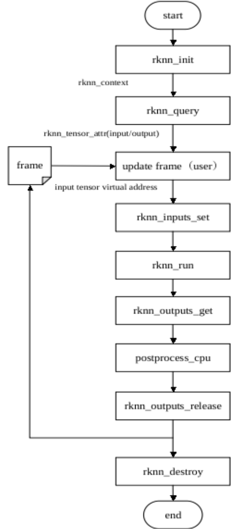
Figure 3-4 The flow chart of general API
Example code of utilizing general API:
// Init RKNN model
ret = rknn_init(&ctx, model, model_len, 0, NULL);

// Get Model Input Output Number
rknn_input_output_num io_num;
ret = rknn_query(ctx, RKNN_QUERY_IN_OUT_NUM, &io_num, sizeof(io_num));

// Get Model Input Info
rknn_tensor_attr input_attrs[io_num.n_input];
memset(input_attrs, 0, sizeof(input_attrs));
for (int i = 0; i < io_num.n_input; i++)
{
  input_attrs[i].index = i;
  ret = rknn_query(ctx, RKNN_QUERY_INPUT_ATTR, &(input_attrs[i]), sizeof(rknn_tensor_attr));
}

// Get Model Output Info
rknn_tensor_attr output_attrs[io_num.n_output];
memset(output_attrs, 0, sizeof(output_attrs));
for (int i = 0; i < io_num.n_output; i++)
{
  output_attrs[i].index = i;
  ret = rknn_query(ctx, RKNN_QUERY_OUTPUT_ATTR, &(output_attrs[i]), sizeof(rknn_tensor_attr));
}

rknn_input inputs[io_num.n_input];
rknn_output outputs[io_num.n_output];
memset(inputs, 0, sizeof(inputs));
memset(outputs, 0, sizeof(outputs));

// Pre-process
// Read Image
image_buffer_t src_image;
memset(&src_image, 0, sizeof(image_buffer_t));
ret = read_image(image_path, &src_image);

// Set Input Data
inputs[0].index = 0;
inputs[0].type = RKNN_TENSOR_UINT8;
inputs[0].fmt = RKNN_TENSOR_NHWC;
inputs[0].size = src_image.size;
inputs[0].buf = src_image.virt_addr;

ret = rknn_inputs_set(rknn_ctx, io_num.n_input, inputs);

// Run
ret = rknn_run(rknn_ctx, nullptr);

// Get Output Data
ret = rknn_outputs_get(rknn_ctx, io_num.n_output, outputs, NULL);

// Post-process
post_process(outputs, results);

// Release RKNN Output
rknn_outputs_release(rknn_ctx, io_num.n_output, outputs);

if (rknn_ctx != 0)
{
  rknn_destroy(rknn_ctx);
}
3.4 Python Inferencing on borad
RKNN-Toolkit Lite2 provides users with a Python interface for board-side model inference, making it convenient for users to use Python language for AI application development.
Note: Before using RKNN-Toolkit Lite2 to develop AI applications, you need to convert the models exported by each deep learning framework into RKNN models through RKNN-Toolkit2. Please refer to Chapter 3.1 for detailed model conversion methods.
3.4.1 Requirement of system environment
The following environment requirements must have to use RKNN-Toolkit Lite2:
Table 3-2 RKNN-Toolkit Lite2 running environment
| OS | Debian 10 / 11 (aarch64) |
|---|---|
| Python version | 3.7 / 3.8 / 3.9 / 3.10 / 3.11 |
| Python dependencies | ‘numpy’ ‘ruamel.yaml’ ‘psutils’ |
3.4.2 Installation of Tools
Please install RKNN-Toolkit Lite2 through the pip3 install command. The installation steps are as follows:
If python3/pip3 and other programs are not installed in the system, please install it through apt-get first. The installation example is as follows:
sudo apt-get update
sudo apt-get install -y python3 python3-dev python3-pip gcc
Note: When installing some dependent modules, you need to compile the source code. At this time, python3-dev and gcc will be used, therefore these two packages are also installed in this step to avoid compilation failure when installing dependent modules later.
Install dependent modules: opencv-python and numpy,example as shown below:
sudo apt-get install -y python3-opencv
sudo apt-get install -y python3-numpy
Note:
1. RKNN-Toolkit Lite2 itself does not rely on opencv-python, but this module needs to be used to process images in this example.
2. Installing numpy through pip3 on Debian10 firmware may fail. It is recommended to use the above method to install it.
Install RKNN-Toolkit Lite2
The installation packages for each platform are placed in the rknn-toolkit-lite2/packages folder of the SDK. Enter the packages folder and execute the following command to install RKNN-Toolkit Lite2:
# Python 3.7
pip3 install rknn_toolkit_lite2-x.y.z-cp37-cp37m-linux_aarch64.whl
# Python 3.8
pip3 install rknn_toolkit_lite2-x.y.z-cp38-cp38-linux_aarch64.whl
# Python 3.9
pip3 install rknn_toolkit_lite2-x.y.z-cp39-cp39-linux_aarch64.whl
# Python 3.10
pip3 install rknn_toolkit_lite2-x.y.z-cp310-cp310-linux_aarch64.whl
# Python 3.11
pip3 install rknn_toolkit_lite2-x.y.z-cp311-cp311-linux_aarch64.whl
3.4.3 Basic flow chart of using RKNN-Toolkit Lite2
The basic process of deploying an RKNN model using RKNN-Toolkit Lite2 is shown in the flow chart below:
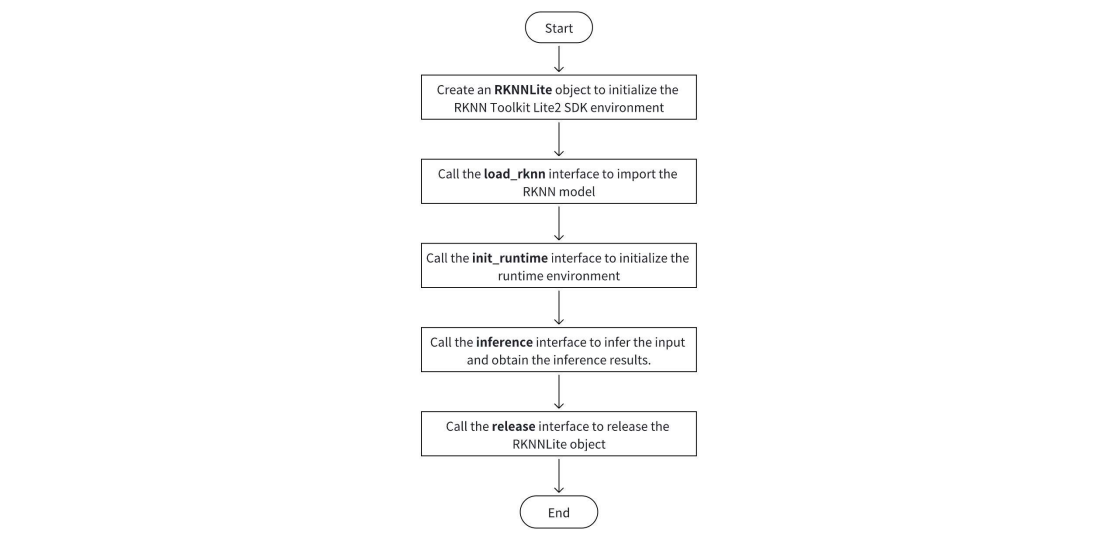
Figure 3-5 the flow chart of RKNN-Toolkit Lite2
Note:
1. Before calling the inference interface for inference, users need to load the input data, perform corresponding preprocessing, and set the parameters in the inference interface based on the input information.
2. After calling the inference interface, the inference results usually need to be processed accordingly to complete upper-layer application-related functions.
3.4.4 Example of running RKNN-Toolkit Lite2
In the directory of SDK/rknn-toolkit-lite2/examples, an image classification application developed based on RKNN-Toolkit Lite2 is provided. The application calls the interface of RKNN-Toolkit Lite2 to load the Resnet18 RKNN model, predict the input image, and print the top5 classification results.
The steps for running this demo:
1. Prepare a development board with RKNN-Toolkit Lite2 installed;
2. Push the directory SDK/rknn-toolkit-lite2/examples to the development board;
3. Go to directory of examples/resent18, executing the following commands to run the demo;
python test.py
The result is shown below:
model: resnet18
-----TOP 5-----
[812]: 0.999676 [class: space shuttle]
[404]: 0.000249 [class: airliner]
[657]: 0.000014 [class: missile]
[833]: 0.000009 [class: bullet train, bullet | submarine, pigboat, sub, U-boat]
[466]: 0.000009 [class: bullet train, bullet | submarine, pigboat, sub, U-boat]
3.4.5 RKNN-Toolkit Lite2 API Detailed Description
This chapter will explain in detail the usage of all APIs provided by RKNN-Toolkit Lite2.
3.4.5.1 RKNNLite Initialization and Release
When using RKNN-Toolkit Lite2, users need to call the RKNNLite() method to initialize an RKNNLite object, and then call the rknn_lite.release() method of the object to release the resources after use.
When initializing the RKNNLite object, users can set the verbose and verbose_file parameters to print detailed log information. The verbose parameter specifies whether to print detailed log information on the screen; if the verbose_file parameter is set and the verbose parameter value is true, the log information will also be written to the file specified by this parameter.
Example code:
# Output detailed log information to the screen and write it to the inference.log file
rknn_lite = RKNNLite(verbose=True, verbose_file='./inference.log')
# Only print detailed log information on the screen
rknn_lite = RKNNLite(verbose=True)
…
rknn_lite.release()
3.4.5.2 Loading RKNN Model
| API | load_rknn |
|---|---|
| Description | Load the RKNN model |
| Parameter | Path to the RKNN model |
| Return | 0: indicating success -1: indicating failed |
Example code:
# Load the resnet18.rknn model from the current directory
ret = rknn_lite.load_rknn('./resnet_18.rknn')
3.4.5.3 Initializing the init_runtime
The init_runtime must call before model inference.
| API | init_runtime |
|---|---|
| Description | Initialize the runtime environment |
| Parameter | core_mask: the specification for NPU core setting. It has the following choices: - RKNNLite.NPU_CORE_AUTO: Referring to automatic mode, meaning that it will select the idle core inside the NPU - RKNNLite.NPU_CORE_0: Running on the NPU0 core - RKNNLite.NPU_CORE_1: Runing on the NPU1 core - RKNNLite.NPU_CORE_2: Runing on the NPU2 core - RKNNLite.NPU_CORE_0_1: Running on both NPU0 and NPU1 core simultaneously - RKNNLite.NPU_CORE_0_1_2: Running on both NPU0, NPU1 and NPU2 simultaneously - RKNNLite.NPU_CORE_ALL: Running on all npu core The default value is NPU_CORE_AUTO, which means the automatic scheduling mode is used by default Note: This parameter is only valid for RK3576/RK3588 |
| Return | 0: indicating success -1: indicating failed |
Example code:
# to initialize the init_runtime
ret = rknn_lite.init_runtime(core_mask=RKNNLite.NPU_CORE_AUTO)
if ret != 0:
  print('Init runtime environment failed')
  exit(ret)
3.4.5.4 Model Inference
| API | inference |
|---|---|
| Description | Perform inference on the specified input and return the inference result |
| Parameter | inputs: input data, such as images read by OpenCV (if the input is four-dimensional, it needs to be manually expanded to 4 dimensions). The type is list, and the list members are ndarray |
| data_format: Data format, type is list, optional values “nhwc”, “nchw” for each input, only valid for four-dimensional input. The default value is None. If this parameter is not filled in, for 4-dimensional input, the data buffer should be arranged according to the NHWC. For non-4-dimensional input, the data buffer should be arranged according to the format required by the model input. If you want to fill in this parameter, for non-4-dimensional input, the data buffer should be arranged according to the format required by the model input (regardless of whether you fill in “nhwc” or “nchw”); for 4-dimensional input, the data buffer should be arranged according to the format set by this parameter. For multi-input models, include all inputs when filling in this parameter |
|
| Return | results: inferencing results with type of python list and its member is type of ndarray |
Using classification as an example, model inference example code shown below:
# Get input data
img = cv2.imread('./space_shuttle_224.jpg')
img = cv2.cvtColor(img, cv2.COLOR_BGR2RGB)
img = np.expand_dims(img, 0)

# Inference
outputs = rknn_lite.inference(inputs=[img])

# Show the classification results
show_top5(outputs)
3.4.5.5 Query SDK version
| API | get_sdk_version |
|---|---|
| Description | Get runtime, driver and RKNN model version information. Note: Model loading and runtime environment initialization must be completed before using this interface. |
| Parameter | None |
| Return | sdk_version: containing information of runtime, driver and RKNN models with type of python string |
Example code:
# Get SDK version information
……
sdk_version = rknn_lite.get_sdk_version()
……
Return information as shown below:
==============================================
RKNN VERSION:
 API: 1.5.2 (71720f3fc@2023-08-21T09:29:52)
 DRV: 0.7.2
==============================================
3.4.5.6 Query available platform for running model
| API | list_support_target_platform |
|---|---|
| Description | Query the chip platform on which the given RKNN model can run |
| Parameter | rknn_model: RKNN model path. If the model path is not specified, the chip platforms currently supported by RKNN-Toolkit Lite2 are printed by category |
| Return | support_target_platform: Returns the chip platform on which the model can run. If the RKNN model path is empty or does not exist, None is returned |
Example code:
rknn_lite.list_support_target_platform(rknn_model=’mobilenet_v1.rknn’)
The result shown below:
**************************************************
Target platforms filled in RKNN model: ['rk3566']
Target platforms supported by this RKNN model: ['RK3566', 'RK3568']
**************************************************
3.5 Matrix Multiplication API
Matmul API is a separate set of C API provided by Runtime, which is used to run matrix multiplication operations on the NPU (RV1103/RV1103B/RV1106/RV1106B/RK2118 does not support it yet). Matrix multiplication is an important operation in linear algebra. The operation is defined as follows:
C=AB,
where A is an M×K matrix, B is a K×N matrix, and C is an M×N matrix.
3.5.1 Features and Usage
The Matmul API is mostly used for parameter calculation tasks in deep learning. For example, matrix multiplication is used extensively in the main modules of the currently widely used Transformer model structure (self-attention mechanism and feedforward neural network layer), so the efficiency of matrix multiplication is crucial to the overall performance of the Transformer model. It has the following characteristics:
Efficient: The bottom layer of Matmul API is implemented using RKNPU, which has the characteristics of high performance and low power consumption.
Flexible: No need to load RKNN models, support int4, int8 and float16 three commonly used input data types for edge computing, provide a separate memory allocation interface or a mechanism to use external memory, and users can manage and reuse the input and output memory of the matrix.
3.5.2 Matmul API Flow Chart
Developers need to include rknn_matmul_api.h header file when compiling their programs since the structure and interface of the Matmul API are located at this header file.
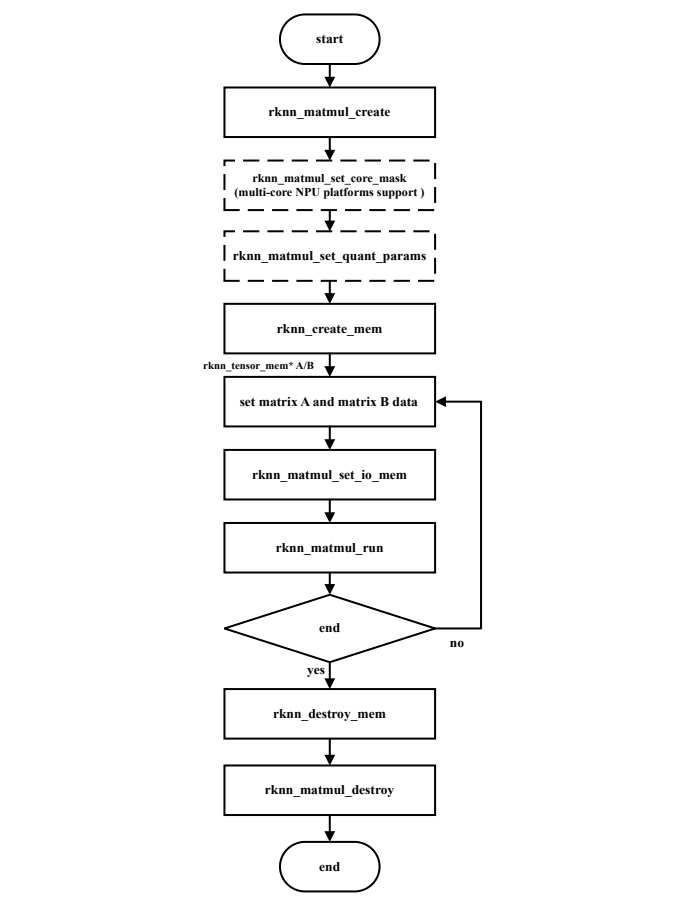
Figure 3-6 The flow chart of basic Matmul API
Steps for using Matmul API:
1. Create context: Set the rknn_matmul_info structure, including M, K, N, the data type of the input and output matrices, the data arrangement used by the input and output matrices, and other information, and then call the rknn_matmul_create interface to initialize the context. After initialization, obtain the rknn_matmul_io_attr structure pointer, which contains the input and output matrix tensor information.
2. Specify the NPU core to run (only valid on multi-core NPU chip platforms): call rknn_matmul_set_core_mask and set the mask to specify a certain NPU core to perform operations. The default behavior of multi-core NPU chip platforms that do not call this interface is to automatically select the idle core.
3. Set the quantization parameters of matrices A, B and C: call rknn_matmul_set_quant_params to pass in the rknn_quant_params structure containing the corresponding matrix quantization parameter values. The default behavior of not calling this interface is scale=1.0, zero_point=0 for each matrix.
4. Creating input and output memory: By calling the rknn_create_mem interface to create memory based on the size of the input and output matrix tensor information.
5. Filling in input data: Fill the data of input matrices A and B according to the shape and data type.And the quantization method sets the quantization parameters.
6. Setting input and output memory: Set input and output memory: Call rknn_matmul_set_io_mem to record the input matrix filled with data into the context, and the output memory is also recorded into the context. In addition to recording the memory address, this interface will also rearrange the data according to the set layout. It must be called after filling or updating the input data. The behavior is different from the rknn_set_io_mem interface in the zero-copy API.
7. Executing matrix multiplication: After finalizing the input and output memory, calling rknn_matmul_run to perform matrix multiplication.
8. Processing output: After performing matrix multiplication, read the result from the output memory according to the set layout.
9. Destroying resources: After execution, calling rknn_destroy_mem and rknn_matmul_destroy to destroy memory and context resources respectively.
3.5.3 Advanced usage of Matmul API
When creating the context, the user is required to set the rknn_matmul_info structure. It represents the specification information used to run matrix multiplication. It includes the size of the matrix multiplication, the data type and data layout of the input and output matrices. Among them, B_layout and AC_layout are used to set high-performance data layouts. The specific structure definition is shown in the following table:
Table 3-3 rknn_matmul_info structure members
| Member | Data Type | Description |
|---|---|---|
| M | int32_t | The number of rows of matrix A |
| K | int32_t | The number of columns of matrix A |
| N | int32_t | The number of columns of matrix B |
| type | rknn_matmul_type | The data types of the input and output matrices: RKNN_FLOAT16_MM_FLOAT16_TO_FLOAT32: Matrix A and B are float16 types, and matrix C is float32 type; RKNN_INT8_MM_INT8_TO_INT32: Indicates that matrices A and B are of type int8, and matrix C is type of int32; RKNN_INT8_MM_INT8_TO_INT8: Indicates that matrices A, B, and C are of type int8; RKNN_FLOAT16_MM_FLOAT16_TO_FLOAT16: Indicates that matrices A, B, and C are of type float16; RKNN_FLOAT16_MM_INT8_TO_FLOAT32: Matrix A is float16, matrix B is int8, and matrix C is float32. RKNN_FLOAT16_MM_INT8_TO_FLOAT16: Matrix A is float16 type, matrix B is int8 type, and matrix C is float16 type; RKNN_FLOAT16_MM_INT4_TO_FLOAT32: Matrix A is float16, matrix B is int4, and matrix C is float32. RKNN_FLOAT16_MM_INT4_TO_FLOAT16: Matrix A is of type float16, matrix B is type int4, and matrix C is type float16; RKNN_INT8_MM_INT8_TO_FLOAT32: Matrix A and B are int8 types, and matrix C is float32 type; RKNN_INT4_MM_INT4_TO_INT16: Indicates that matrices A and B are int4 types, and matrix C is int16 types; RKNN_INT8_MM_INT4_TO_INT32: Matrix A is of type int8, type B is type int4, and matrix C is type int32 |
| B_layout | int16_t | How the data is arranged in Matrix B. RKNN_MM_LAYOUT_NORM: Matrix B is arranged according to the original shape, i.e., the shape of KxN; RKNN_MM_LAYOUT_NATIVE: Matrix B is arranged according to high-performance shapes; RKNN_MM_LAYOUT_TP_NORM: Indicates that matrix B is arranged according to the shape after Transpose, that is, the shape of NxK |
| B_quant_type | int16_t | The type of quantization method of matrix B. RKNN_QUANT_TYPE_PER_LAYER_SYM: Matrix B is symmetrically quantized according to the Per-Layer method; RKNN_QUANT_TYPE_PER_LAYER_ASYM: Matrix B is asymmetrically quantized according to the Per-Layer method. RKNN_QUANT_TYPE_PER_CHANNEL_SYM: Matrix B is symmetrically quantized according to the Per-Channel mode. RKNN_QUANT_TYPE_PER_CHANNEL_ASYM: Matrix B is asymmetrically quantized according to the Per-Channel method. RKNN_QUANT_TYPE_PER_GROUP_SYM: Representation matrix B is symmetrically quantized according to the Per-Group method; RKNN_QUANT_TYPE_PER_GROUP_ASYM: Matrix B is asymmetrically quantified according to the Per-Group method |
| AC_layout | int16_t | How the data is arranged for matrices A and C. RKNN_MM_LAYOUT_NORM: Indicates that matrices A and C are arranged according to their original shapes; RKNN_MM_LAYOUT_NATIVE: Represents matrices A and C arranged in high-performance shapes The specification can be referred to 3.5.4 |
| AC_quant_type | int16_t | How the data is arranged for matrices A and C. RKNN_MM_LAYOUT_NORM: Indicates that matrices A and C are arranged according to their original shapes; RKNN_MM_LAYOUT_NATIVE: Represents matrices A and C arranged in high-performance shapes |
| iommu_domain_id | int32_t | Index of the IOMMU address space domain where the matrix context resides. The IOMMU address space corresponds to the context one-to-one, and the size of each IOMMU address space is 4GB. This parameter is mainly used when the parameter specifications of matrices A, B, and C are large, and the memory allocated by the NPU in a certain domain exceeds 4GB and needs to be switched to another domain. |
| group_size | int16_t | The number of elements in a group takes effect only when group quantization is enabled. |
| reserved | int8_t[] | Reserved fields |
The original shape of matrix A is MxK, the original shape of matrix B is KxN, and the original shape of matrix C is MxN.
3.5.3.1 Matrix multiplication with specified quantization parameters
If the high-bit data of the matrix product needs to be quantized into low-bit data according to the quantization parameter, for example, matrices A and B are of type int8, and matrix C is of type int8, you need to set the quantization parameters of the matrix. The quantization parameters consist of scale and zero_point, use rknn_quant_params The structure indicates that the quantization parameters of matrices A and C are set through the rknn_matmul_set_quant_params interface. After the quantization parameters are set successfully, the quantization parameters of matrix B in Per-Channel quantization mode can be read through the rknn_matmul_get_quant_params interface. The rknn_quant_params data structure definition is shown in the following table:
Table 3-4 rknn_quant_params structure definition
| Member | Data Type | Description |
|---|---|---|
| name | char[] | The name of matrix |
| scale | float* | The first address of the quantization parameter scale array |
| scale_len | int32_t | The length of the quantization parameter scale array |
| zp | int32_t* | The first address of the quantization parameter zero_point array |
| zp_len | int32_t | The length of the quantization parameter zero_point array |
There are three quantization methods of Matmul: Per-Layer, Per-Channel, and Per-Group, and the quantization parameters are as follows:
Per-Layer method: The length of the scale and zp arrays is 1.
Per-Channel method: The scale and zp arrays are of N length.
Per-Group mode: The length of the scale and zp arrays is N*K/group_size, the number of elements in each group is specified by group_size, and the elements in the same group share the same quantization parameters group_size.
There are two ways of symmetric quantization and asymmetric quantization, symmetric quantization means that zp is all 0, and asymmetric quantization means that zp is not all 0.
3.5.3.2 Matrix multiplication of dynamic shape input
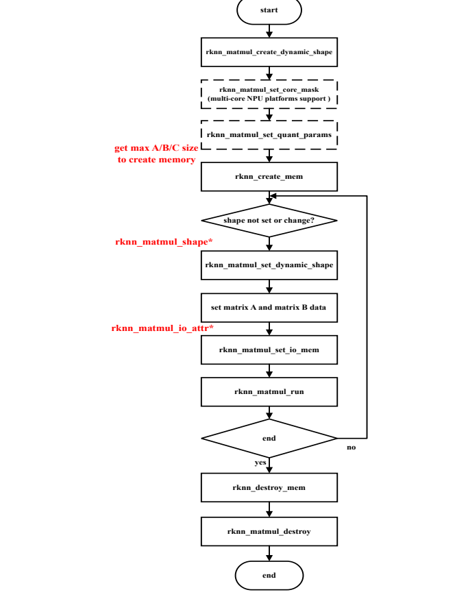
Figure 3-7 Matmul API calling process for dynamic shape input
The flow of Matmul API usage for dynamic shape input is shown in the figure above. The process differences between using the dynamic shape Matmul API and the basic Matmul API are as follows:
1. Create a context: configure the number of shapes and required shapes, and set the rknn_matmul_info structure, which contains information such as the data type of the input and output matrices, the data arrangement used by the input and output matrices, and other information. Note that M, K, and N in the dynamic shape Matmul interface parameter rknn_matmul_info do not need to be set. Then, call the rknn_matmul_create_dynamic_shape interface to initialize the context. After initialization, obtain the
rknn_matmul_io_attr structure array, which contains input and output matrix Tensor information under all shape configurations.
2. Create input and output memory: First obtain the maximum Tensor size from the rknn_matmul_io_attr structure array, call the rknn_create_mem interface, and create memory using the maximum input and output matrix Tensor size.
3. Set the input shape: By calling the rknn_matmul_set_dynamic_shape interface and passing in the rknn_matmul_shape pointer, set the shape used in the current inference process.
4. Set input and output memory: Call rknn_matmul_set_io_mem to record the input matrix filled with data into the context, and the output memory is also recorded into the context. The passed-in rknn_tensor_mem* parameter is the input and output memory of the maximum size created previously, and the rknn_matmul_tensor_attr* parameter is the matrix attribute information corresponding to the current shape.
3.5.4 The data layout for high-performance
Since the NPU is a dedicated hardware architecture, it is not the most efficient to read the original shape data of MxK and KxN. Similarly, it is not the most efficient to write the C matrix of MxN shape. Users can use special data arrangement methods to achieve more efficient results to achieve high performance. The AC_layout parameter controls whether matrices A and C use the high-performance data layout, and the B_layout parameter controls whether matrix B uses the high-performance data layout.
Assuming that the original shape of matrix A is MxK, matrix B is KxN and matrix C is MxN. The required data layout is as follows:
1. If AC_layout=RKNN_MM_LAYOUT_NORM and B_layout=RKNN_MM_LAYOUT_NORM, the shape of matrix A is [M,K], the shape of matrix B is [K,N], and the shape of matrix C is [M,N].
2. If AC_layout=RKNN_MM_LAYOUT_NATIVE and B_layout=RKNN_MM_LAYOUT_NATIVE, the high-performance data of matrices A, B, and C under different chip platforms and data types are arranged in the following table (the division results in the table are rounded up, and the extra part is filled with 0):
3. The difference between B_layout=RKNN_MM_LAYOUT_NORM and B_layout=RKNN_MM_LAYOUT_TP_NORM is that the former matrix B is in the shape of [K,N], and the latter matrix B is in the shape of [N,K], and the latter is more efficient in execution.
Table 3-5 High-performance shapes for individual chip platform matrices A, B, and C
| Shape | RK3562 | RK3566/RK3568 | RK3576/RV1126B | RK3588 |
|---|---|---|---|---|
| A(int4) | unsupported | unsupported | [K/32,M,32] | [K/32,M,32] |
| B(int4) | unsupported | unsupported | [N/64,K/32,64,32]* | [N/64,K/32,64,32] |
| C(int16) | unsupported | unsupported | [N/8,M,8] | [N/8,M,8] |
| A(int8) | [K/16,M,16] | [K/8, M, 8] | [K/16,M,16] | [K/16,M,16] |
| B(int8) | [N/16,K/32,16,32] | [N/16,K/32,16,32] | [N/32,K/32,32,32]* | [N/32,K/32,32,32] |
| C(int32) | [N/4,M,4] | [N/4,M,4] | [N/4,M,4] | [N/4,M,4] |
| A(float16) | [K/8,M,8] | [K/4,M,4] | [K/8,M,8] | [K/8,M,8] |
| B(float16) | [N/8,K/32,8,32] | [N/8,K/16,8,16] | [N/16,K/32,16,32] | [N/16,K/32,16,32] |
| C(float32) | [N/4,M,4] | [N/4,M,4] | [N/4,M,4] | [N/4,M,4] |
Note
The data in the above table is arranged in the same type as A and B (i.e., A and B are of the same data type). The RK3576/RV1126B supports “different type” inputs, i.e. allowing A and B to have different data types, and in the case of “different types” of inputs, B’s high-performance data arrangement is the same as that of B in the “same type” case corresponding to Type C. For example, if A is of type int4, B is of type float16, and C is of type float32, then the data arrangement of B’s high-performance data is [N/16,K/32,16,32]. The ‘rknn_B_normal_layout_to_native_layout’ interface provides the ability to convert the original shape of B into a high-performance arrangement.
Using the RK3566/RK3568 platform and the int8 data type as an example, the element relationship of matrix A transformed from [M,K] to [K/8,M,8] is as shown in the figure below:
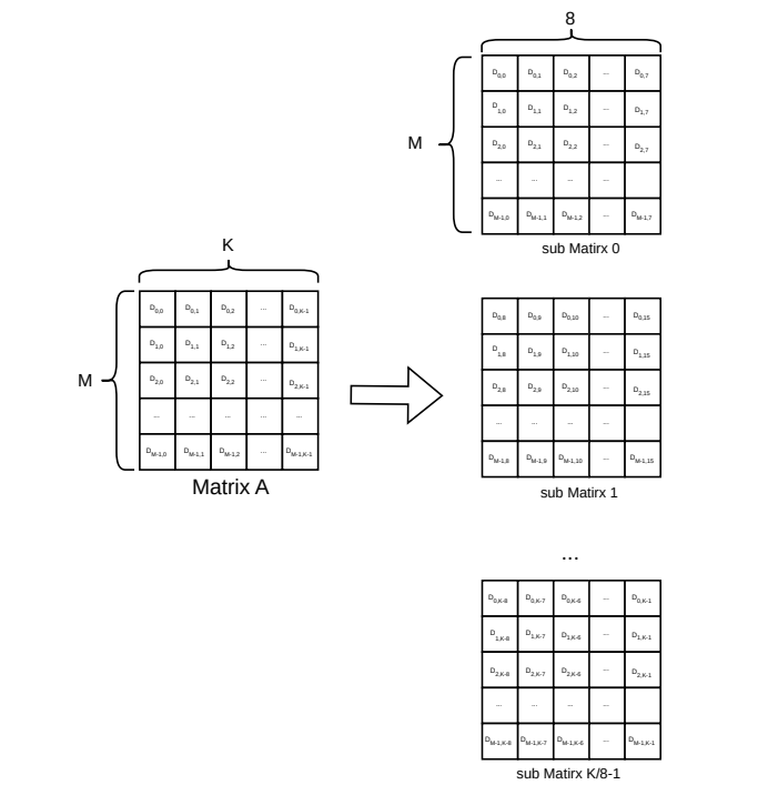
Figure 3-8 The element correspondence diagram of int8 type matrix A transformed from [M,K] to [K/8,M,8]
The data corresponding to the (i, j)-th element of matrix A is Di, j. The left picture is a matrix with shape=[M,K], and each sub-matrix in the right picture has shape=[M,8], from top to bottom, with the number of K/8 submatrices in total.
The example code for converting matrix A or C from original shape to high-performance shape is as follows:
template <typename Ti, typename To>
void norm_layout_to_perf_layout(Ti *src, To *dst, int32_t M, int32_t K, int32_t subK)
{
  int outter_size = (int)std::ceil(K * 1.0f / subK);
  for (int i = 0; i < outter_size; i++)
  {
    for (int m = 0; m < M; m++)
    {
      for (int j = 0; j < subK; j++)
      {
        int ki = i * subK + j;
        if (ki >= K)
        {
          dst[i * M * subK + m * subK + j] = 0;
        }
        else
        {
          dst[i * M * subK + m * subK + j] = src[m * K + ki];
        }
      }
    }
  }
}
Based on the RK3566/RK3568 platform, the element correspondence of matrix B of int8 data type transformed from [K, N] to [N/16, K/32, 16, 32] is shown in the figure below:
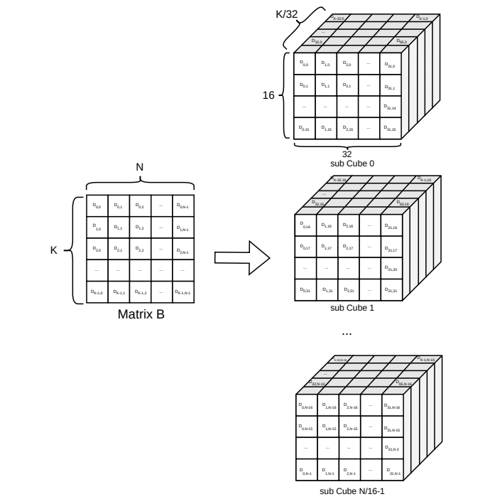
Figure 3-9 The element correspondence diagram of the int8 type matrix B transformed from [K, N] to [N/16, K/32, 16, 32]
The data corresponding to the (i, j) element of matrix B is Di, j. The left picture is a matrix with shape=[K, N], and each small cube in the right picture has shape=[K/32,16,32]. There are N/16 in total from top to bottom.
The example code for converting matrix B from its original shape to a high-performance shape is as follows:
template <typename Ti, typename To>
void norm_layout_to_native_layout(Ti *src, To *dst, int32_t K, int32_t N, int32_t subN, int32_t subK)
{
  int N_remain = (int)std::ceil(N * 1.0f / subN);
  int K_remain = (int)std::ceil(K * 1.0f / subK);
  for (int i = 0; i < N_remain; i++)
  {
    for (int j = 0; j < K_remain; j++)
    {
      for (int n = 0; n < subN; n++)
      {
        int ni = i * subN + n;
        for (int k = 0; k < subK; k++)
        {
          int ki = j * subK + k;
          if (ki < K && ni < N)
          {
            dst[((i * K_remain + j) * subN + n) * subK + k] = src[ki * N + ni];
          }
          else
          {
            dst[((i * K_remain + j) * subN + n) * subK + k] = 0;
          }
        }
      }
    }
  }
}
Note
The full Matmul API example code can be seen by this link. https://github.com/airockchip/rknn-toolkit2/tre e/master/rknpu2/examples/rknn_matmul_api_demo
3.5.4.1 Matrix specification restrictions
The Matmul API is an NPU-based hardware architecture implementation and is subject to hardware specifications.There are the following limitations on the parameters:
AC_layout and B_layout can be set independently. RKNN_MM_LAYOUT_NORM or RKNN_MM_LAYOUT_TP_NORM are supported on AC_layout and B_layout on all hardware platforms, and RKNN_MM_LAYOUT_TP_NORM are supported on all platforms except the RK3566/RK3568 platform.
The MATMUL interface supports a variety of input and output data bit widths, and the matrix data types supported by each platform are combined in the following table:
Table 3-6 Data types of matrices A, B, and C supported by the Matmul interface
| Serial number | RK3562 | RK3566/RK3568 | RK3576/RV1126B | RK3588 |
|---|---|---|---|---|
| 1 | RKNN_INT8_MM_INT8_TO_INT32 | RKNN_INT8_MM_INT8_TO_INT32 | RKNN_FLOAT16_MM_FLOAT16_TO_FLOAT16 | RKNN_FLOAT16_MM_FLOAT16_TO_FLOAT16 |
| 2 | RKNN_FLOAT16_MM_FLOAT16_TO_FLOAT32 | RKNN_FLOAT16_MM_FLOAT16_TO_FLOAT32 | RKNN_FLOAT16_MM_FLOAT16_TO_FLOAT32 | RKNN_FLOAT16_MM_FLOAT16_TO_FLOAT32 |
| 3 | RKNN_INT8_MM_INT8_TO_INT32 | RKNN_INT8_MM_INT8_TO_INT32 | ||
| 4 | RKNN_FLOAT16_MM_INT8_TO_FLOAT32 | RKNN_INT8_MM_INT8_TO_FLOAT32 | ||
| 5 | RKNN_FLOAT16_MM_INT4_TO_FLOAT16 | RKNN_INT8_MM_INT8_TO_INT8 | ||
| 6 | RKNN_FLOAT16_MM_INT4_TO_FLOAT32 | RKNN_INT4_MM_INT4_TO_INT16 | ||
| 7 | RKNN_INT8_MM_INT4_TO_INT32 |
The float16 floating point format follows the IEEE-754 standard. Please refer to the specific format IEEE-754 half
The restriction sizes for K and N are as follows:
Table 3-7 Size limitations of K and N for each chip platform
| RK3562 | RK3566/RK3568 | RK3576/RV1126B | RK3588 | |
|---|---|---|---|---|
| K size limit (int4) |
not supported | not supported | * | 32 aligned |
| K size limit (int8) |
K <= 10240 and K mod 32 = 0 |
K <= 10240 and K mod 32 = 0 |
32 aligned | 32 aligned |
| K size limit (float16) |
K <= 10240 and K mod 32 = 0 |
K <= 10240 and K mod 32 = 0 |
32 aligned | 32 aligned |
| N size limit (int4) |
not supported | not supported | * | N <= 8192 and N mod 64 = 0 |
| N size limit (int8) |
N <= 4096 and N mod 16 = 0 |
N <= 4096 and N mod 16 = 0 |
N <= 4096 and N mod 32 = 0 |
N <= 4096 and N mod 32 = 0 |
| N size limit (float16) |
N <= 4096 and N mod 16 = 0 |
N <= 4096 and N mod 16 = 0 |
N <= 4096 and N mod 32 = 0 |
N <= 4096 and N mod 32 = 0 |
Note
* indicates that the size and alignment limits are the same as those of B corresponding to the data type A on the same platform. For example, RKNN_FLOAT16_MM_INT4_TO_FLOAT32 combination type B has the same size and alignment limits as RKNN_FLOAT16_MM_FLOAT16_TO_FLOAT32 combination.
for RK3588:
when K > 8192, the B data will be split into T segments.
int T = std::ceil(K / 8192);
For example: normal layout -> native layout K = 20488, N = 4096, T = 3, the data will be split into 3 segments.
subN = rknn_matmul_io_attr.B.dims[2];
subK = rknn_matmul_io_attr.B.dims[3];
The shape of K,N during conversion,
                     (8196, 4096) (4096 / subN, 8196 / subK, subN, subK)
 (K, N) = (20488, 4096)->(8196, 4096)->(4096 / subN, 8196 / subK, subN, subK)
         normal layout (4096, 4096) (4096 / subN, 4096 / subK, subN, subK)
                   T normal layout T native layout
It is recommended to use the rknn_B_normal_layout_to_native_layout interface for direct data conversion.
for RK3576/RV1126B:
when K > 4096, the B data will be split into T segments.
int T = std::ceil(K / 4096);
For example: normal layout -> native layout K = 10240, N = 2048, T = 3, the data will be split into 3 segments.
subN = rknn_matmul_io_attr.B.dims[2];
subK = rknn_matmul_io_attr.B.dims[3];
The shape of K,N during conversion,
                        (4096, 2048) (2048 / subN, 4096 / subK, subN, subK)
(K, N) = (10240, 2048) -> (4096, 2048) -> (2048 / subN, 4096 / subK, subN, subK)
        normal layout (2048, 2048) (2048 / subN, 2048 / subK, subN, subK)
                     T normal layout T native layout
It is recommended to use the rknn_B_normal_layout_to_native_layout interface for direct data conversion.
4 Example
RKNN provides examples of different models, including MobileNet, YOLOv5, etc. The code project is located in the https://github.com/airockchip/rknn_model_zoo/tree/main/examples directory.
The following operations take RK3588 Linux platform, Ubuntu22.04 and Python3.8 in Conda environment as examples. For the installation of the development environment, please refer to Chapter 2. For the deployment process of other platforms, please refer to <Rockchip_RKNPU_Quick_Start_RKNN_SDK>.
4.1 Model Deployment Example: MobileNet
This chapter takes MobileNet model deployment as an example to introduce how to quickly get started with model conversion, model running with board, model evaluation, and model board deployment.
4.1.1 Model Conversion
1. Switch to the rknn_model_zoo/examples/mobilenet/python directory:
cd rknn_model_zoo/examples/mobilenet/python
2. Execute model conversion and perform image inference:
python mobilenet.py --model ../model/mobilenetv2-12.onnx --target rk3588
After executing this command, the model will perform inference on the computer simulator. The converted model is saved by default at the path rknn_model_zoo/examples/mobilenet/model/mobilenet_v2.rknn.
4.1.2 Model Running with Device
1. Switch to the rknn_model_zoo/examples/mobilenet/python directory:
cd rknn_model_zoo/examples/mobilenet/python
2. Run the model on the device:
python mobilenet.py --target rk3588 --npu_device_test
After executing this command, the model performs inference on the device.
The output is as follows:
-----TOP 5-----
[494] score=0.99 class="n03017168 chime, bell, gong"
[469] score=0.00 class="n02939185 caldron, cauldron"
[653] score=0.00 class="n03764736 milk can"
[747] score=0.00 class="n04023962 punching bag, punch bag, punching ball, punchball"
[505] score=0.00 class="n03063689 coffeepot"
4.1.3 Model Evaluation
RKNN provides (simulator and on-device) accuracy evaluation, time-consuming evaluation and memory evaluation functions to assist in the optimization and deployment of RKNN models.
4.1.3.1 Accuracy Evaluation
1. Switch to the rknn_model_zoo/examples/mobilenet/python directory:
cd rknn_model_zoo/examples/mobilenet/python
2. Perform model accuracy analysis:
python mobilenet.py --target rk3588 --accuracy_analysis --npu_device_test
The output results of the model accuracy analysis are as follows:
# simulator_error: calculate the output error of each layer of the simulator (compared to the 'golden' value).
# entire: output error of each layer between 'golden' and 'simulator', these errors will accumulate layer by layer.
# single: single-layer output error between 'golden' and 'simulator', can better reflect the single-layer accuracy of the simulator.
layer_name simulator_error
                  entire single
                cos euc cos euc
---------------------------------------------------------------
...
[Conv] 464 0.99202 | 4.1079 0.99998 | 0.1981
[Conv] output_conv 0.99308 | 13.235 0.99992 | 1.4133
[Reshape] output_int8 0.99308 | 13.235 0.99993 | 1.3043
[exDataConvert] output 0.99308 | 13.235 0.99993 | 1.3043

# runtime_error: calculate the output error of each layer of the runtime.
# entire: output error of each layer between 'golden' and 'runtime', these errors will accumulate layer by layer.
# single_sim: single-layer output error between 'simulator' and 'runtime', can better reflect the single-layer accuracy of runtime.
layer_name runtime_error
                  entire single_sim
                cos euc cos euc
---------------------------------------------------------------
...
[Conv] 464 0.99210 | 4.2718 1.00000 | 0.0
[Conv] output_conv 0.99203 | 14.847 1.00000 | 0.2007
[Reshape] output_int8
[exDataConvert] output 0.99203 | 14.847 1.00000 | 0.0
4.1.3.2 Time-consuming Evaluation
1. Switch to the rknn_model_zoo/examples/mobilenet/python directory:
cd rknn_model_zoo/examples/mobilenet/python
2. Perform model time-consuming evaluation:
python mobilenet.py --target rk3588 --eval_perf
The output results of the model time-consuming evaluation are as follows:
---------------------------------------------------------------
    Network Layer Information Table
---------------------------------------------------------------
ID OpType DataType Target Time(us) ...
---------------------------------------------------------------
1 InputOperator UINT8 CPU 17
2 ConvClip UINT8 NPU 331
3 ConvClip INT8 NPU 429
4 Conv INT8 NPU 292
....
55 Conv INT8 NPU 374
56 Reshape INT8 CPU 61
57 OutputOperator INT8 CPU 11
---------------------------------------------------------------
Total Operator Elapsed Per Frame Time(us): 12631
Total Memory Read/Write Per Frame Size(KB): 10563
---------------------------------------------------------------

---------------------------------------------------------------
    Operator Time Consuming Ranking Table
---------------------------------------------------------------
OpType CallNumber ... NPUTime(us) TotalTime(us) TimeRatio(%)
---------------------------------------------------------------
ConvClip 35 8436 8436 66.79%
Conv 9 2093 2093 16.57%
ConvAdd 10 2013 2013 15.94%
Reshape 1 0 61 0.48%
InputOperator 1 0 17 0.13%
OutputOperator 1 0 11 0.09%
---------------------------------------------------------------
4.1.3.3 Memory Evaluation
1. Switch to the rknn_model_zoo/examples/mobilenet/python directory:
cd rknn_model_zoo/examples/mobilenet/python
2. Perform model memory evaluation:
python mobilenet.py --target rk3588 --eval_memory
The output results of the model memory evaluation are as follows:
---------------------------------------------------------------
    Network Layer Information Table
---------------------------------------------------------------
ID OpType DataType Target Time(us) ...
---------------------------------------------------------------
1 InputOperator UINT8 CPU 17
2 ConvClip UINT8 NPU 331
3 ConvClip INT8 NPU 429
4 Conv INT8 NPU 292
....
55 Conv INT8 NPU 374
56 Reshape INT8 CPU 61
57 OutputOperator INT8 CPU 11
---------------------------------------------------------------
Total Operator Elapsed Per Frame Time(us): 12631
Total Memory Read/Write Per Frame Size(KB): 10563
---------------------------------------------------------------

---------------------------------------------------------------
    Operator Time Consuming Ranking Table
---------------------------------------------------------------
OpType CallNumber ... NPUTime(us) TotalTime(us) TimeRatio(%)
---------------------------------------------------------------
ConvClip 35 8436 8436 66.79%
Conv 9 2093 2093 16.57%
ConvAdd 10 2013 2013 15.94%
Reshape 1 0 61 0.48%
InputOperator 1 0 17 0.13%
OutputOperator 1 0 11 0.09%
---------------------------------------------------------------
4.1.4 Model Deployment on the Device
1. Specify the gcc cross-compiler path in the build-linsx.sh script under the rknn_model_zoo project:
GCC_COMPILER=~/opts/gcc-linaro-6.3.1-2017.05-x86_64_aarch64-linux-gnu/bin/aarch64-linux-gnu
For information on how to download and install the gcc cross-compiler, please refer to <Rockchip_RKNPU_Quick_Start_RKNN_SDK>.
2. Compilation
cd rknn_model_zoo
./build-linux.sh -t rk3588 -a aarch64 -d mobilenet
3. Push the executable file to the board:
adb push install/rk3588_linux_aarch64/rknn_mobilenet_demo /userdata/
4. Run the model on the device:
adb shell

cd /userdata/rknn_mobilenet_demo
export LD_LIBRARY_PATH=./lib
./rknn_mobilenet_demo model/mobilenet_v2.rknn model/bell.jpg
The output is as follows:
-----TOP 5-----
[494] score=0.993227 class=n03017168 chime, bell, gong
[469] score=0.002560 class=n02939185 caldron, cauldron
[747] score=0.000466 class=n04023962 punching bag, punch bag, punching ball, punchball
[792] score=0.000466 class=n04208210 shovel
[618] score=0.000405 class=n03633091 ladle
4.2 Model Deployment Example: YOLOv5
4.2.1 Model Conversion
1. Download model.
cd rknn_model_zoo/examples/yolov5/model
./download_model.sh
2. Perform model conversion:
cd rknn_model_zoo/examples/yolov5/python
python convert.py ../model/yolov5s_relu.onnx rk3588 i8 ../model/yolov5.rknn
The converted model save path is rknn_model_zoo/examples/yolov5/model/yolov5.rknn.
4.2.2 Model Running with Device
1. Switch to the rknn_model_zoo/examples/yolov5/python directory:
cd rknn_model_zoo/examples/yolov5/python
2. Run the model on the device:
python yolov5.py --model_path ../model/yolov5.rknn --target rk3588 --img_show
The default input image is model/bus.jpg, and the result image is as follows:
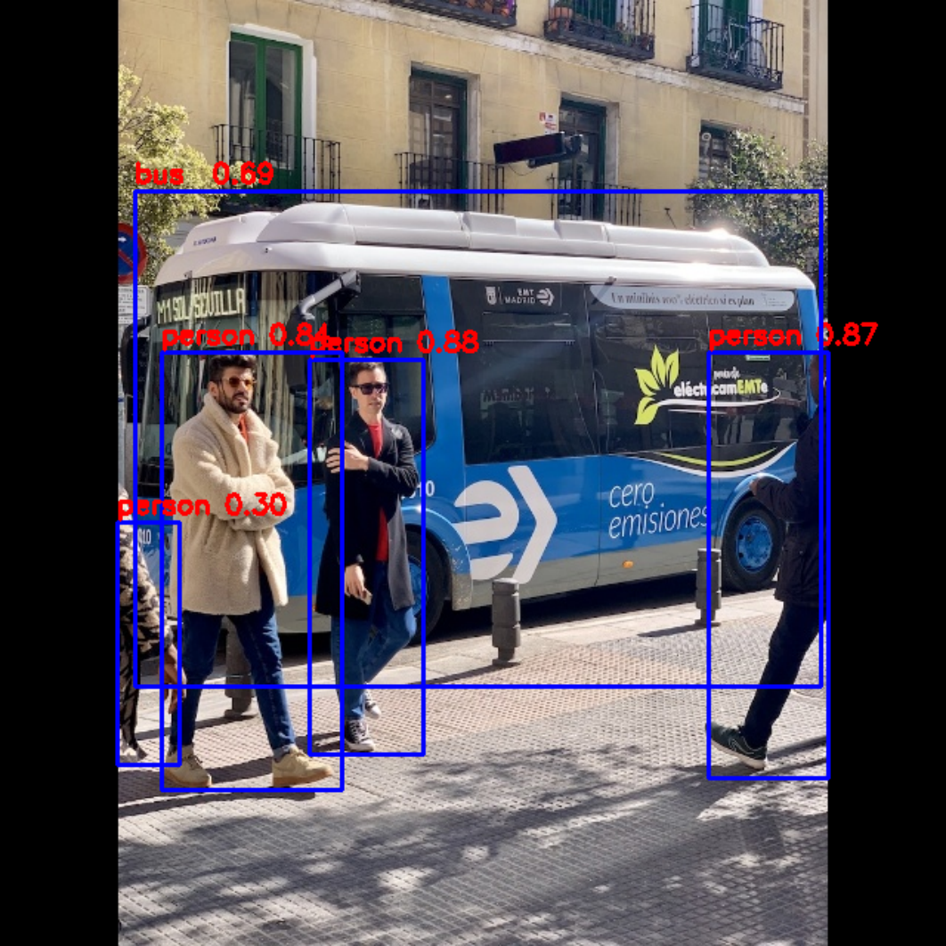
Figure 4-1 RKNN output image of python demo
4.2.3 Model Deployment on the Device
1. Specify the gcc cross-compiler path in the build-linsx.sh script under the rknn_model_zoo project:
GCC_COMPILER=~/opts/gcc-linaro-6.3.1-2017.05-x86_64_aarch64-linux-gnu/bin/aarch64-linux-gnu
For information on how to download and install the gcc cross-compiler, please refer to <Rockchip_RKNPU_Quick_Start_RKNN_SDK>.
2. Compilation:
cd rknn_model_zoo
./build-linux.sh -t rk3588 -a aarch64 -d yolov5
3. Push the executable file to the device:
adb push install/rk3588_linux_aarch64/rknn_yolov5_demo /userdata/
4. Run the model on the device:
adb shell
cd userdata/rknn_yolov5_demo
export LD_LIBRARY_PATH=./lib
./rknn_yolov5_demo model/yolov5.rknn model/bus.jpg
5. Pull it from the board end and view it locally. In the terminal of the local computer, execute the following command:
adb pull /userdata/rknn_yolov5_demo/out.png .
The output image is as follows:
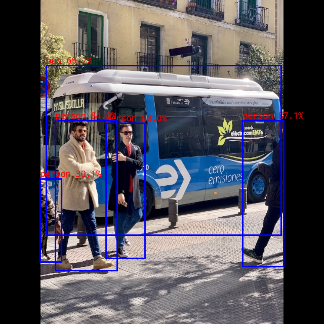
Figure 4-2 RKNN output image of C demo
5 RKNN Advanced Instructions
5.1 Data Formats
Currently, there are four data formats of RKNN: NHWC, NCHW, NC1HWC2, and UNDEFINE. The data format of NHWC and NCHW is a common data format for deep learning, therefore will not provide additional explanations. This chapter focuses on the storage and conversion of the NC1HWC2 data format dedicated to RKNPU hardware.
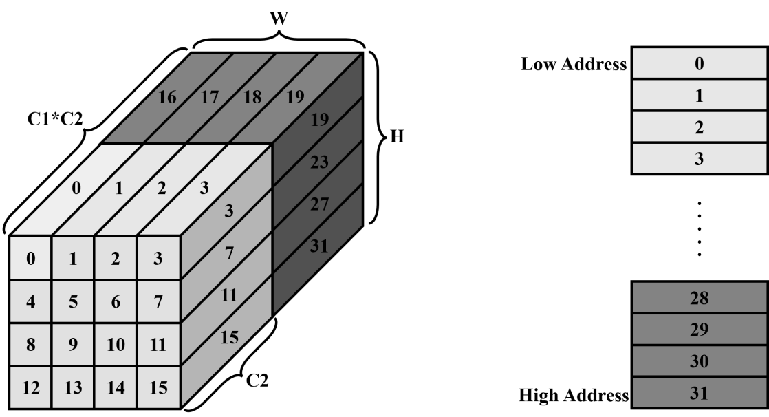
Figure 5-1 RKNPU NC1HWC2 data format and storage
As shown in Figure 5-1, the number 0 represents the storage of C2 data block, where C2 is determined by the platform. The rule constraints of C2 on different RKNPU hardware platforms are as shown in Table 5-1, and C1 is the rounded-up value of C/C2. The order of NC1HWC2 data storage is consistent with the order of numerical growth in the Figure 5-1. Data from 0-15 is stored first, and then data from 16-31 is stored. Take the RK3568 platform as an example, the corresponding NC1HWC2 is (1, 2, 4, 4, 8) when the int8 feature data is (1, 13, 4, 4). In this case, C2 is 8, C1 is 2. And for the C2 data block of 16-31, only the first five data of each corresponding C2 data blocks are valid, the remaining three data are additional aligned invalid data.
Table 5-1 C2 on different RKNPU hardware platforms
| RV1103/RV1106 | RV1103B/RV1106B | RK2118 | RK3562 | RK3566/RK3568 | RK3576/RK3588/RV1126B | |
|---|---|---|---|---|---|---|
| int8 | 16 | 8 | / | 16 | 8 | 16 |
| float16 | 8 | / | 4 | 8 | 4 | 8 |
Next, we will introduce the process of converting NC1HWC2 data format into NCHW and NHWC data formats in memory. Take the RK3568 platform as an example, according to the previous alignment requirements the corresponding NC1HWC2 is (1, 2, 2, 2, 8) when the int8 feature data is (1, 13, 2, 2). The storage of NC1HWC2 is as shown in the figure below, wherein the red parts are additional aligned invalid data.
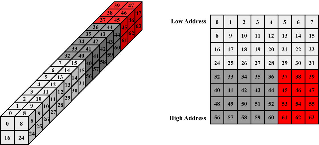
Figure 5-2 NC1HWC2 data arrangement expansion
Remove invalid data and convert into NCHW, that is, (1, 13, 2, 2) format data which is arranged in the memory as follows:
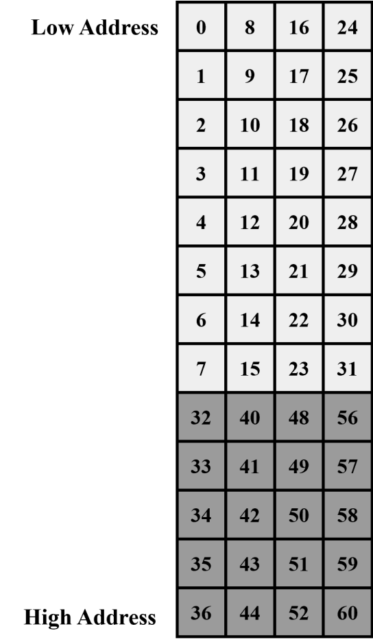
Figure 5-3 NCHW layout
Remove invalid data and convert into NHWC, that is, (1, 2, 2, 13) format data which is arranged in the memory as follows:
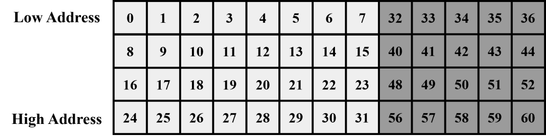
Figure 5-4 NHWC layout
The sample code for conversion is as follows:
1.NC1HWC2 to NCHW: Convert NC1HWC2 with int8 data format to NCHW with int8 data
/*
 *src: represents the address of NC1HWC2 tensor
 *dst: represents the address of the NCHW tensor
 *dims: represents the shape information of NC1HWC2
 *channel: represents the value of C in NCHW
 * h : represents the value of h in NCHW
 * w: represents the value of w in NCHW
 */
int NC1HWC2_to_NCHW(const int8_t* src, int8_t* dst, int* dims, int channel, int h, int w)
{
  int batch = dims[0];
  int C1 = dims[1];
  int C2 = dims[4];
  int hw_src = dims[2] * dims[3];
  int hw_dst = h * w;
  for (int i = 0; i < batch; i++) {
    src = src + i * C1 * hw_src * C2;
    dst = dst + i * channel * hw_dst;
    for (int c = 0; c < channel; ++c) {
    int plane = c / C2;
    const int8_t* src_c = plane * hw_src * C2 + src;
    int offset = c % C2;
    for (int cur_h = 0; cur_h < h; ++cur_h)
      for (int cur_w = 0; cur_w < w; ++cur_w) {
      int cur_hw = cur_h * w + cur_w;
      dst[c * hw_dst + cur_h * w + cur_w] = src_c[C2 * cur_hw + offset];
      }
    }
  }

  return 0;
}
2.NC1HWC2 to NHWC: Convert NC1HWC2 with int8 data format to NHWC with int8 data
/*
 *src: represents the address of NC1HWC2 tensor
 *dst: represents the address of the NCHW tensor
 *dims: represents the shape information of NC1HWC2
 *channel: represents the value of C in NCHW
 * h : represents the value of h in NCHW
 * w: represents the value of w in NCHW
 */
int NC1HWC2_to_NHWC(const int8_t* src, int8_t* dst, int* dims, int channel, int h, int w)
{
  int batch = dims[0];
  int C1 = dims[1];
  int C2 = dims[4];
  int hw_src = dims[2] * dims[3];
  int hw_dst = h * w;
  for (int i = 0; i < batch; i++) {
    src = src + i * C1 * hw_src * C2;
    dst = dst + i * channel * hw_dst;
    for (int cur_h = 0; cur_h < h; ++cur_h) {
      for (int cur_w = 0; cur_w < w; ++cur_w) {
        int cur_hw = cur_h * dims[3] + cur_w;
        for (int c = 0; c < channel; ++c) {
          int plane = c / C2;
          const auto* src_c = plane * hw_src * C2 + src;
          int offset = c % C2;
          dst[cur_h * w * channel + cur_w * channel + c] = src_c[C2 * cur_hw + offset];
        }
      }
    }
  }
  return 0;
}
5.2 RKNN Runtime Zero-Copy Interface
5.2.1 Zero-Copy Introduction
There are two groups of APIs that can be used on RK3562/RK3566/RK3568/RK3576/RK3588/RV1126B, namely the general API interface and the zero-copy API interface, but RV1103/RV1103B/RV1106/RV1106B only support the zero-copy API interface. For zero-copy example code, please refer to the examples/rknn_zero_copy directory under the rknpu2 project. For detailed information and code library of rknpu2, please visit the link: https://github. com/airockchip/rknn-toolkit2/tree/master/rknpu2.
When inferring the RKNN model, the original data must go through three major processes: input processing, NPU running model, and output processing. Currently, according to different model input formats and quantification methods, there are two processing processes within the interface: general API and zero-copy API, as shown in
Figure 5-5 and Figure 5-6.The main difference between the two APIs is that each time the general interface updates the frame data, the data allocated externally needs to be copied to the input memory of the NPU during runtime, while the zero-copy interface uses preallocated memory directly (including memory created by NPU or other frame, such as DRM), reducing the cost of copying memory, better performance and less bandwidth. When the user input data has only virtual address, only the general API interface can be used; when the user input data has a physical address or fd, both sets of interfaces can be used. General API and zero-copy API interface cannot be called together.
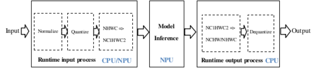
Figure 5-5 Data processing flow of general API
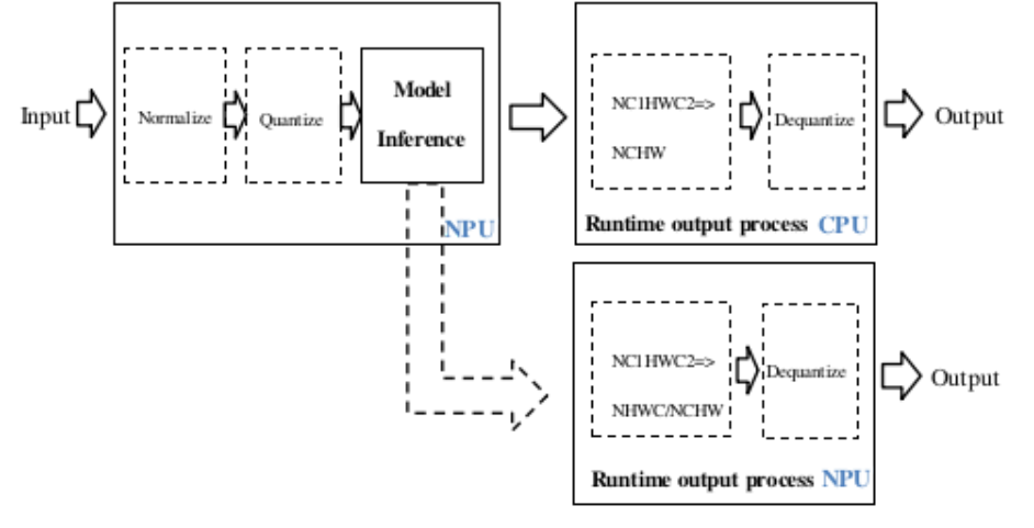
Figure 5-6 Data processing flow of zero-copy API
General API
The processing flow of the general API is shown in Figure 5-5. The normalization, quantification, data format conversion, and dequantization of data are running on the CPU except for the inference of the model which runs on the NPU (When alignment requirements for zero-copy input are met, normalization and quantization will run on the NPU, but the input data still needs to be copied to the model’s input buffer using the CPU).
Zero-copy API
The processing flow of the zero-copy API is shown in Figure 5-6. The data processing flow of the general API is optimized. Zero-copy API normalization, quantization, and model inference are all running on the NPU. The output data format and dequantization process is running on the CPU or NPU. The zero-copy API will process the input data flow more efficiently than the general API.
The conditions for the zero-copy scenario are as shown in the following table:
Table 5-2 Zero-Copy input alignment requirements
| Input dimensions | Input alignment requirements | |
|---|---|---|
| RV1103B/RV1106B/RK3566/RK3568 | RV1103/RV1106/RV1126B/RK3562/RK3576/RK3588 | |
| 4 dimensions, the number of channels is 1, 3, 4 |
Width 8-byte aligned | Width 16-byte aligned |
| Not 4 dimensions | Total size 8-byte aligned | Total size 16-byte aligned |
5.2.2 C API Zero-Copy Process
The zero-copy API interface uses the rknn_tensor_memory structure, it’s necessary to create and set the structure before inference, and read the memory information in the structure after inference. According to whether the user needs to allocate the modular memory of model (input/output/weights/internal result) and the different memory representation (file descriptor/physical address, etc.), there are the following three typical zero copy calling processes, as shown in Figure 5-7 to Figure 5-9. The red font indicates the interface and data structure specially added for zero copy and the italic indicates the data structure passed between interface calls.
1. Input/Output memory is allocated during runtime
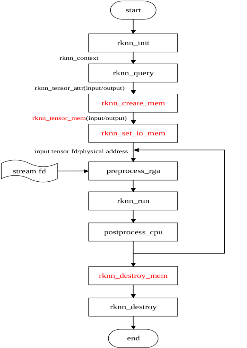
Figure 5-7: The process of zero copy API interface (input/output allocated internally)
As shown in Figure 5-7, the input/output memory allocated by the runtime is called rknn_create_mem() interface to create the rknn_tensor_memory structure, and rknn_set_io_mem() sets the input and output rknn_tensor_memory structure.
The input/output memory information structure created by the rknn_create_mem() interface contains file descriptor and physical addresses. The RGA interface uses the memory information allocated by the NPU, preprocess_rga() represents the RGA interface, and stream_fd represents the RGA interface input source buffer, postprocess_cpu()represents the CPU implementation of postprocessing.
2. Input/output memory is allocated externally
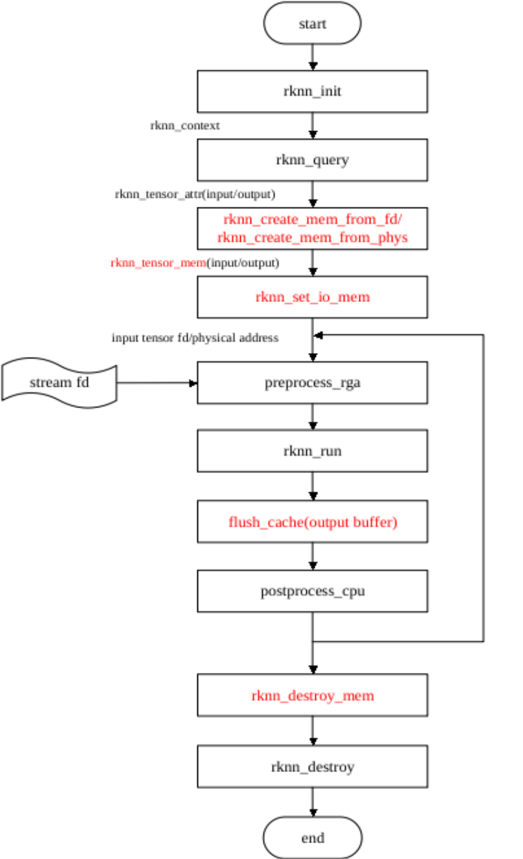
Figure 5-8 The process zero-copy API interface (input/output allocated externally)
As shown in Figure 5-8, the input/output memory is called by external allocation using the rknn_create_mem_from_fd()/rknn_create_mem_from_phys() interface to create the rknn_tensor_memory structure, and rknn_set_io_mem() to set the input and output rknn_tensor_memory structure, flush_cache indicates that the user needs to call the interface associated with the allocated memory type to flush the output cache.
3. Input/output/weights/internal tensor memory is allocated externally
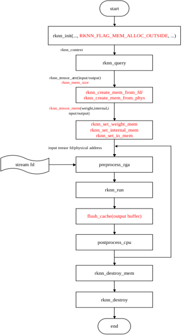
Figure 5-9 The process of zero copy API interface (input/output/weights/internal tensor allocated externally)
As shown in Figure 5-9, the input/output/weight/internal result memory is allocated externally by the rknn_create_mem_from_fd()/rknn_create_mem_from_phys() interface to create the rknn_tensor_memory structure, and rknn_set_io_mem() sets the input and output rknn_tensor_memory structure, rknn_set_weight_mem()/rknn_set_internal_mem() sets the weight/internal result rknn_tensor_memory structure.
5.2.3 C API Zero-Copy Usage
Taking Figure 5-6 the process of zero copy API interface (input/output allocated internally) as an example, the usage is as follows:
rknn_query()
Input:
Use RKNN_QUERY_NATIVE_INPUT_ATTR to query related attributes (note, not RKNN_QUERY_INPUT_ATTR). When the format (or layout) queried is different, the way to preprocess is also different. The input layout and type queried in this way are the optimal hardware efficiency.
The input situation of rknn_query() is as follows:
1. When the layout is RKNN_TENSOR_NCHW, the input is generally 4 dimensional and the data type is bool or int64. When transfering data to the NPU, it also needs to be arranged in the NCHW format.
2. When the layout is RKNN_TENSOR_NHWC, the input is generally 4 dimensional and the data type is one of the float32/float16/int8/uint8. And the number of input channels is 1, 3 or 4. When transfering data to the NPU, it also needs to be arranged in the NHWC format and sent to the NPU. It should be noted that when pass_through=1, the width may need to be aligned with stride, depending on the value of w_stride queried.
3. When the layout is RKNN_TENSOR_NC1HWC2, the input is generally 4-dimensional and the data type is float16/int8. And the number of input channels is not 1, 3, or 4. When pass_through=0, the input data is arranged in the NHWC format, and the interface will perform CPU conversion from NHWC to NC1HWC2; when pass_through=1, the input data is arranged in the NC1HWC2 format, and the user needs to convert it externally.
4. When the layout is RKNN_TENSOR_UNDEFINED, the input is generally not 4-dimensional. When transfering data to the NPU, it needs to be passed to the NPU according to the input format of ONNX model. NPU does not perform any mean/std processing and layout conversion.
If the input configuration required by the user is different from the rknn_tensor_attr structure obtained by the query interface, the rknn_tensor_attr structure can be modified. The currently supported modifiable input data types are shown in Table 5-3. Special attention: If the data type of the query is uint8, but the user wants to pass in float32 type, the size of the rknn_tensor_attr structure must be modified to four times the original size, and the data type must be modified to RKNN_TENSOR_FLOAT32. After modification in this way, the hardware efficiency is not optimal, and the CPU will be called internally in the interface to perform data type conversion.
Table 5-3 Input modifiable data type table
| The input data type obtained by rknn_query |
|||||||
|---|---|---|---|---|---|---|---|
| bool | int8 | float16 | int16 | int32 | int64 | ||
| The input data type modified by user |
bool | Y | |||||
| int8 | Y | ||||||
| uint8 | Y | Y | |||||
| float32 | Y | Y | |||||
| float16 | Y | ||||||
| int16 | Y | ||||||
| int32 | Y | ||||||
| int64 | Y |
Output:
Use RKNN_QUERY_NATIVE_OUTPUT_ATTR to query related attributes (note, not RKNN_QUERY_OUTPUT_ATTR). When the format (or layout) queried is different, the way to preprocess is also different. The output layout and type queried in this way are the optimal hardware efficiency.
When the output is 4-dimensional and the user needs NHWC layout output, can use RKNN_QUERY_NATIVE_NHWC_OUTPUT_ATTR to query related attributes. This way can directly query native output nhwc layout from NPU.
The output situation of rknn_query() is as follows:
1. When the layout is RKNN_TENSOR_NC1HWC2, the output is generally 4-dimensional and the
data type is float16/int8. When the user requires NCHW layout, conversion from NC1HWC2 to NCHW needs to be performed externally.
2. When layout is RKNN_TENSOR_UNDEFINED, the output is generally not 4-dimensional, and the
data type is float16/int8. The user no need to perform layout conversion externally.
3. When layout is RKNN_TENSOR_NCHW, the output is generally 4-dimensional, and the data type is
float16/int8. The user no need to perform layout conversion externally.
4. When the layout is RKNN_TENSOR_NHWC, the output is generally 4-dimensional and the data
type is float16/int8. This situation is usually caused by the user calling the RKNN_QUERY_NATIVE_NHWC_OUTPUT_ATTR interface to query the layout.
If the output configuration required by the user is different from the rknn_tensor_attr structure obtained by the query interface, the rknn_tensor_attr structure can be modified. The modifiable configuration information is shown in Table 5-4 and Table 5-5. Special attention: If the data type of the query output is int8, and the user wants to obtain the float32 type output, the size of the rknn_tensor_attr structure must be modified to four times the original size, and the data type must be modified to RKNN_TENSOR_FLOAT32. After modification in this way, the hardware efficiency is not optimal, and the CPU will be called internally in the interface to perform data type conversion.
Table 5-4 Output modifiable data type table
| The output data type obtained by rknn_query |
|||||||
|---|---|---|---|---|---|---|---|
| bool | int8 | float16 | int16 | int32 | int64 | ||
| The output data type modified by user |
bool | Y | |||||
| int8 | Y | ||||||
| uint8 | |||||||
| float32 | Y | Y | |||||
| float16 | Y | ||||||
| int16 | Y | ||||||
| int32 | Y | ||||||
| int64 | Y |
Table 5-5 Output layout type
| The output layout obtained by rknn_query |
|||||
|---|---|---|---|---|---|
| NC1HWC2 | NCHW | NHWC | UNDEFINED | ||
| The output layout set by user |
NC1HWC2 | Y | |||
| NCHW | Y | Y | |||
| NHWC | Y | ||||
| UNDEFINED | Y |
The zero-copy interface NPU output configuration supported by RK3562/RK3566/RK3568/RK3576/RK3588/RV1126B is shown in Table 5-6. The zero-copy interface NPU output configuration supported by RV1103/RV1103B/RV1106/RV1106B is shown in Table 5-7.
Table 5-6 Output configurations supported by RK3562/RK3566/RK3568/RK3576/RK3588/RV1126B zero- copy interface NPU
| Model type | Output data type | Output dimensions | Supported output layout |
|---|---|---|---|
| int8 Model | int8/float16/float32 | 4 dimensions | NCHW/NC1HWC2/NHWC |
| Not 4 dimensions | UNDEFINE | ||
| float16 Model | float16/float32 | 4 dimensions | NCHW/NC1HWC2/NHWC |
| Not 4 dimensions | UNDEFINE |
Table 5-7 Output configurations supported by RV1103/RV1103B/RV1106/RV1106B zero-copy interface NPU
| Model type | Output data type | Output dimensions | Supported output layout |
|------------|------------------|-------------------|-------------------------|
| int8 Model | int8/float16 | 4 dimensions | NCHW/NC1HWC2/NHWC |
| | | Not 4 dimensions | UNDEFINE |
rknn_create_mem
The zero-copy API interface uses the rknn_tensor_memory structure, need to create and set the structure before inference, and read the memory information in the structure after inference. When there is no need to modify the layout and type from RKNN_QUERY_NATIVE_INPUT_ATTR, RKNN_QUERY_NATIVE_OUTPUT_ATTR, the default configured size_with_stride is used directly to create the memory size. If the corresponding layout and type are modified, the memory size needs to be created according to the corresponding size. (For example, the output data type is int8. If the user wants to obtain float32 type output, the size must be modified to four times the original size)
rknn_set_io_mem
rknn_set_io_mem() is used to set the rknn_tensor_mem structure containing model input/output memory information. Similar to rknn_init(), you only need to call it once at the beginning, and then execute rknn_run() repeatedly.
5.3 NPU Multi-Core Configuration
RK3588 provides stronger computing power through 3 core NPU, RK3576 provides stronger computing power through 2 core NPU. This chapter will introduce in detail the configuration method of multi-core NPU to improve the inference efficiency of the model.
Note: Multi-core operation is suitable for networks with a large amount of calculations. A little improvement for small networks, and may even lead to performance degradation due to single-core and multi-core switching (this switching requires CPU intervention).
5.3.1 Multi-Core Operation Configuration Method
If you use Python as the application development language, you can set the NPU core for model running through the “core_mask” parameter in the init_runtime() interface of RKNN-Toolkit2 or RKNN-Toolkit Lite2. The detailed description of this parameter is as follows:
If you use Python as the application development language, you can set the NPU core for model running through the “core_mask” parameter in the init_runtime() interface of RKNN-Toolkit2 or RKNN-Toolkit Lite2. The detailed description of this parameter is as follows:
Table 5-8 init_runtime interface core_mask parameter description
| Parameter | Description |
|---|---|
| core_mask | Sets the NPU cores at model runtime. The supported configurations are as follows: - NPU_CORE_AUTO: Indicates the automatic scheduling model, which automatically runs on the currently idle NPU Core. - NPU_CORE_0: Model running on the NPU Core0. - NPU_CORE_1: Model running on the NPU Core1. - NPU_CORE_2: Model running on the NPU Core2. - NPU_CORE_0_1: Model running on the NPU Core0 and Core1 at the same time. - NPU_CORE_0_1_2: Model running on the NPU Core0, Core1 and Core2 at the same time. - NPU_CORE_ALL: Selecting the number of NPU cores to run depending on the platform. The default value is NPU_CORE_AUTO. Note: When setting this parameter on RKNN-Toolkit Lite2, RKNNLite must be added in front of the value, such as RKNNLite.NPU_CORE_AUTO; if this parameter is set on RKNN-Toolkit2, RKNN must be added in front of the value, such as RKNN.NPU_CORE_AUTO. |
RKNN-Toolkit2 sets the NPU core. The reference code is as follows:
# Init runtime environment
print('--> Init runtime environment')
ret = rknn.init_runtime(target='rk3588', core_mask=RKNN.NPU_CORE_0)
if ret != 0:
  print('Init runtime environment failed!')
  exit(ret)
print('done')
RKNN-Toolkit Lite2 sets the NPU core. The reference code is as follows:
......
# Init runtime environment
print('--> Init runtime environment')
ret = rknn_lite.init_runtime(core_mask=RKNNLite.NPU_CORE_0)
if ret != 0:
  print('Init runtime environment failed')
  exit(ret)
print('done')
......
If you use C/C++ as the application development language, you can call the rknn_set_core_mask() interface to set the NPU core for model running. The detailed description of the interface core_mask is as follows:
Table 5-9 rknn_set_core_mask interface core_mask parameter description
| Parameter | Description |
|---|---|
| core_mask | Sets the NPU cores at model runtime. The supported configurations are as follows: - RKNN_NPU_CORE_AUTO: Indicates the automatic scheduling model, which automatically runs on the currently idle NPU Core. - RKNN_NPU_CORE_0: Model running on the NPU Core0. - RKNN_NPU_CORE_1: Model running on the NPU Core1. - RKNN_NPU_CORE_2: Model running on the NPU Core2. - RKNN_NPU_CORE_0_1: Model running on the NPU Core0 and Core1 at the same time. - RKNN_NPU_CORE_0_1_2: Model running on the NPU Core0, Core1 and Core2 at the same time. - RKNN_NPU_CORE_ALL: Selecting the number of NPU cores to run depending on the platform. |
Use the C/C++ API to set up the model running on the NPU core. The reference code is as follows:
// rknn_context ctx;
rknn_core_mask core_mask = RKNN_NPU_CORE_0;
int ret = rknn_set_core_mask(ctx, core_mask);
5.3.2 Check Multi-Core Running Status
This chapter will detail the effect of the RKNN model when running in multi-core mode.
If you use RKNN-Toolkit2 to connect to the RKNPU device for model inference, you need to set the perf_debug parameter to True when calling the rknn.init_runtime()interface, and then call the rknn.eval_perf() interface to print the running information of each layer. The reference code is as follows:
# Init runtime environment
ret = rknn.init_runtime(target='rk3588', device_id='29d5dd97766a5c27', perf_debug=True)
if ret != 0:
  print('Init runtime environment failed!')
  exit(ret)

# Eval performance
rknn.eval_perf()
If you perform model inference directly on the device, you need to set RKNN_LOG_LEVEL to 4 or above before running the application. The running information of each layer of the model will be printed. The setting method is as follows:
# Using the python interface provided by RKNN-Toolkit Lite2, just set verbose to True when creating the RKNNLite object.
rknnlite = RKNNLite(verbose=True)

# Using the C/C++ interface, you need to set the following environment variables before running the binary program
export RKNN_LOG_LEVEL=4
Taking the lenet model as an example, after passing the above settings, the terminal will print a log similar to the following (for the convenience of display, InputShape, OutputShape, DDR Cycles, NPU Cycles, Total Cycles, Time(us), MacUsage(%), Task Number, Lut Number, RW(kb), FullName and other fields have been deleted):
ID OpType DataType Target WorkLoad(0/1/2)-ImproveTherical
1 InputOperator UINT8 CPU 100.0%/0.0%/0.0% - Up:0.0%
2 Conv UINT8 NPU 50.0%/50.0%/0.0% - Up:50.0%
3 MaxPool INT8 NPU 100.0%/0.0%/0.0% - Up:0.0%
4 Conv INT8 NPU 50.0%/50.0%/0.0% - Up:50.0%
5 MaxPool INT8 NPU 100.0%/0.0%/0.0% - Up:0.0%
6 ConvRelu INT8 NPU 48.1%/51.9%/0.0% - Up:48.1%
7 Conv INT8 NPU 100.0%/0.0%/0.0% - Up:0.0%
8 Softmax INT8 CPU 0.0%/0.0%/0.0% - Up:0.0%
9 OutputOperator FLOAT16 CPU 0.0%/0.0%/0.0% - Up:0.0%
Total Operator Elapsed Time(us): 591
Total Memory RW Amount(MB): 0
The “WorkLoad(0/1/2)-ImproveTherical” column in the running information of each layer of the model is only printed on multi-core NPUs. It records how the tasks of each layer of the model are allocated on the NPU core and its theoretical performance improvement. For example, “50.0%/50.0%/0.0% - Up:50.0%” means that the calculation amount of this layer is distributed with Core0 responsible for 50% and Core1 responsible for 50%. Compared with single-core operation, the performance of this layer can theoretically be improved by 50%. If the performance of a certain layer has not improved, such as “100.0%/0.0%/0.0% - Up:0.0%”, the following situations may exist:
The load of this layer is too small, smaller than the granularity of NPU multi-core task allocation, so this layer runs on a single core;
This type of operator does not implement multi-core task segmentation in the NPU driver and will be supported in subsequent versions. The existing operators that support multi-core task segmentation include: Conv, DepthwiseConvolution, Add, Concat, Relu, Clip, Relu6, ThresholdedRelu, PRelu, and LeakyRelu.
5.3.3 Multi-Core Performance Improvement Tips
You can try the following methods to get higher multi-core running performance:
Set CPU/DDR/NPU frequency to the highest
Bind the application to the CPU big core
Bind the NPU interrupt to the corresponding CPU big core above
The fixed frequency commands corresponding to different firmware are different, please refer to Chapter 8.1.1.
Take binding the application to the CPU4 core as an example. For the last two points mentioned above, you can refer to the following script:
interrupts=$(cat /proc/interrupts | grep npu)
interrupts_array=($interrupts)

irq1=$(echo ${interrupts_array[0]} | awk -F ':' '{print $1}')
irq2=$(echo ${interrupts_array[14]} | awk -F ':' '{print $1}')
irq3=$(echo ${interrupts_array[28]} | awk -F ':' '{print $1}')

for irq in $irq1 $irq2 $irq3; do
 echo 4 > /proc/irq/$irq/smp_affinity_list
done

taskset 10 ./rknn_benchmark lenet.rknn "" 10 3 # The taskset mask value corresponding to CPU4 is 0x10
The above script will perform the following operations:
Execute the cat /proc/interrupts | grep npu command and parse out three interrupt numbers (remove colons)
Use a loop to set the smp_affinity_list of each interrupt number to 4 (the corresponding ID of CPU4 is 4)
Finally execute the taskset 10 ./rknn_benchmark lenet.rknn “” 10 3 command. The taskset parameter corresponding to CPU4 is 10 (For specific usage of taskset, please refer to: https://man7.org/linux/man-page s/man1/taskset.1.html)
Through the above operation, the NPU interrupt and the application “rknn_benchmark” will run on CPU4, which can eliminate the core switching overhead of NPU interrupt processing.
5.4 Dynamic Shape
5.4.1 Dynamic Shape Introduction
Dynamic shape means that the shape of the model input data can change at runtime. It can help handle situations where the input data size is not fixed and increase the flexibility of the model. In the case of the RKNN model that only supported static shape before, if the user needs to use multiple input shapes, the traditional approach is to generate multiple RKNN models and initialize multiple contexts to perform inference separately when deploying the model. However, after the introduction of dynamic shape, can only keep a copy of the dynamic shape RKNN model that is similar in size to the static shape RKNN model, and use one context for inferenceing, thus saving Flash and DDR occupancy. Dynamic shape plays an important role in image processing and sequence model reasoning. Typical application scenarios include:
Models with changing sequence lengths, common in NLP models, such as BERT, GPT
Models that vary in spatial dimensions, such as segmentation and style transfer
The model with batch, the batch dimension changes
Object detection model with variable output number
5.4.2 RKNN SDK Version and Platform Requirements
RKNN-Toolkit2 version>=1.5.0
RKNPU Runtime library (librknnrt.so) version >=1.5.0
The RK3562/RK3566/RK3568/RK3576/RK3588/RV1126B platform supports this function
5.4.3 Generate RKNN Model of Dynamic Shape
This chapter introduces the steps to generate an RKNN model with dynamic shape using the python interface of RKNN-Toolkit2:
1. Confirm that the model supports dynamic shape
If the model file itself is not a dynamic shape, RKNN-Toolkit2 supports RKNN models expanded into dynamic shape. First, the user must confirm that the model itself does not have operators or subgraph structures that limit dynamic shape. For example, the shape of the constant cannot be changed, the RKNN- Toolkit2 tool will report an error during the conversion process. If dynamic shape expansion is not supported, according to the error message, the users modify the model structure and retrain the model to support dynamic shape. It is recommended to use a model that is a dynamic shape.
2. Set the input shape to be used
Due to NPU hardware characteristics, the dynamic shape RKNN model does not support arbitrary changes in input shapes and requires users to set a limited number of input shapes. For multi-input models, the number of shapes for each input must be the same. For example, when using RKNN-Toolkit2 to convert a Caffe model, the python code example is as follows:
dynamic_input = [
  [[1,3,224,224]], # set the first shape for all inputs
  [[1,3,192,192]], # set the second shape for all inputs
  [[1,3,160,160]], # set the third shape for all inputs
]

# Pre-process config
rknn.config(mean_values=[103.94, 116.78, 123.68], std_values=[58.82, 58.82, 58.82],
      quant_img_RGB2BGR=True, dynamic_input=dynamic_shapes)
The above interface configuration will generate a dynamic shape RKNN model that supports three shapes: [1,3,224,224], [1,3,192,192] and [1,3,160,160]. The shape in dynamic_input is consistent with the layout of the original model frame. For example, for classified RGB images of the same size 224x224, the TensorFlow/TFLite model input is [1,224,224,3], while the ONNX model input is [1,3,224,224].
3. Quantization
After setting the input shape, if you want to quantize, you need to set the quantization calibration dataset. The toolkit will read the maximum resolution input set by the user for quantization (the largest set of shapes that is the sum of all input sizes). For example, the model has two inputs, one input shape is [1,224] and [1,112], and the other input shape is [1,40] and [1,80] respectively. The sum of all input dimensions for the first group shapes is 1224+140=264, the sum of all input sizes for the second group shapes is 1112+180=192, the sum of all the input sizes for the first group shapes is larger, so ues the two inputs of [1,224] and [1,40] to quantize.
If the quantization calibration dataset is in jpg/png format, the user can use images of different resolutions for quantification, because the toolkit will use the resize method of opencv to scale the image to the maximum resolution before quantizing it.
If the quantization calibration dataset is in npy format, the user must use the maximum resolution input shape. After quantization, all shapes in the model use the same set of quantization parameters for inference at runtime.
In addition, the maximum resolution input shape will also be printed when calling rknn.config, as follows:
W config: The 'dynamic_input' function has been enabled, the MaxShape is dynamic_input[0] = [[1,224],[1,40]]!
The following functions are subject to the MaxShape:
1. The quantified dataset needs to be configured according to MaxShape
2. The eval_perf or eval_memory return the results of MaxShape
4. Inference or Accuracy Analysis
When using the dynamic shape RKNN model for inference or accuracy analysis, the user must provide one of the set of shapes input in step 2. The interface usage is consistent with the static shape RKNN model, and will not be described in detail here.
For a complete example of creating a dynamic shape RKNN model, please refer to (https://github.com/airoc kchip/rknn-toolkit2/tree/master/rknn-toolkit2/examples/functions/dynamic_shape)
5.4.4 C API Deployment
After obtaining the dynamic shape RKNN model, use the RKNPU2 C API to deploy it. According to the interface form, it is divided into general API and zero-copy API deployment processes.
5.4.4.1 General API
The process of deploying a dynamic shape RKNN model using a general API is shown in the figure below:
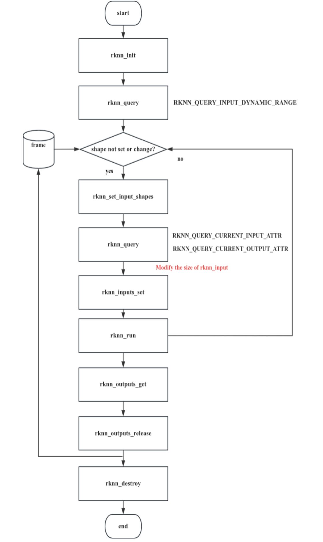
Figure 5-10 General API calling process of dynamic shape input interface)
After loading the dynamic shape RKNN model, the input shape can be dynamically modified at runtime. First, the input shape list supported by the RKNN model can be queried through rknn_query(). The shape list information supported by each input is returned in the form of the rknn_input_range structure, which contains the name of each input, data layout information, number of shapes, and specific shapes. Next, by calling the rknn_set_input_shapes() interface and passing in the rknn_tensor_attr array pointer containing each input shape information to set the shape used for current inference. Then you can call rknn_query() again to query the input and output shapes after the successful setting.
Finally, the inference is completed according to the general API process. Each time you switch the input shape, you need to set a new shape, prepare data of the new shape and call the rknn_inputs_set() interface again. If there is no need to switch input shapes before inference, there is no need to call the rknn_set_input_shapes() interface repeatedly.
1. Initialization
Call the rknn_init() interface to initialize the dynamic shape RKNN model.
For the dynamic shape RKNN model, there are the following restrictions when initializing the context:
Weight sharing function is not supported(initialization with RKNN_FLAG_SHARE_WEIGHT_MEM flag).
The context reuse function is not supported (see the rknn_dup_context interface for details).
2. Query the input shape list supported by the RKNN model
After successful initialization, the input shape list supported by the RKNN model can be queried through rknn_query(). The shape list information supported by each input is returned in the form of the rknn_input_range structure, which contains the name of each input, layout information, the numbers of shapes and specific shapes. The C code example is as follows:
// Query the input shape supported by the model
rknn_input_range dyn_range[io_num.n_input];
memset(dyn_range, 0, io_num.n_input * sizeof(rknn_input_range));
for (uint32_t i = 0; i < io_num.n_input; i++)
{
  dyn_range[i].index = i;
  ret = rknn_query(ctx, RKNN_QUERY_INPUT_DYNAMIC_RANGE, &dyn_range[i],
sizeof(rknn_input_range));
  if (ret != RKNN_SUCC)
  {
    fprintf(stderr, "rknn_query error! ret=%d\n", ret);
    return -1;
  }
  dump_input_dynamic_range(&dyn_range[i]);
}
Note: For multi-input models, all input shapes correspond one-to-one in order. For example, in an RKNN model with two inputs and multiple shapes, the first shape of the first input and the first shape of the second input combinations are valid, and there are no intersecting shape combinations. For example, the model has two inputs A and B. The shapes of A are [1,224] and [1,112] respectively, and the shapes of B are [1,40] and [1,80] respectively. At this time, only the following two cases of input shapes are supported:
A shape = [1,224], B shape=[1,40]
A shape = [1,112], B shape=[1,80]
3. Set input shape
When input data is set for the first time or the input shape changes, the rknn_set_input_shapes() interface needs to be called to dynamically modify the input shape. After loading the dynamic shape RKNN model, the input shape can be dynamically modified at runtime. By calling the rknn_set_input_shapes() interface, pass in the rknn_tensor_attr array of all inputs. The three member information(dims, n_dims and fmt) in each rknn_tensor_attr represents the shape of the current inference. The C code example is as follows:
/**
 dynamic inputs shape range:
 index=0, name=data, shape_number=2, range=[[1, 224, 224, 3],[1, 112, 224, 3]], fmt = NHWC
**/
input_attrs[0].dims[0] = 1;
input_attrs[0].dims[1] = 224;
input_attrs[0].dims[2] = 224;
input_attrs[0].dims[3] = 3;
input_attrs[0].fmt=RKNN_TENSOR_NHWC;
ret = rknn_set_input_shapes(ctx, io_num.n_input, input_attrs);
if (ret < 0) {
  fprintf(stderr, "rknn_set_input_shapes error! ret=%d\n", ret);
  return -1;
}
Among io_num.n_input is the number of inputs, and input_attrs is the rknn_tensor_attr structure array of model input.
Note: The shape set here must be included in the shape list queried in step 2.
After setting the input shape, can call rknn_query again to query the input and output shapes that current setting is successful. The C code example is as follows:
// Get the input and output shape of the current inference
rknn_tensor_attr cur_input_attrs[io_num.n_input];
memset(cur_input_attrs, 0, io_num.n_input * sizeof(rknn_tensor_attr));
for (uint32_t i = 0; i < io_num.n_input; i++)
{
  cur_input_attrs[i].index = i;
  ret = rknn_query(ctx, RKNN_QUERY_CURRENT_INPUT_ATTR, &(cur_input_attrs[i]),
sizeof(rknn_tensor_attr));
  if (ret < 0)
  {
    printf("rknn_init error! ret=%d\n", ret);
    return -1;
  }
  dump_tensor_attr(&cur_input_attrs[i]);
}

rknn_tensor_attr cur_output_attrs[io_num.n_output];
memset(cur_output_attrs, 0, io_num.n_output * sizeof(rknn_tensor_attr));
for (uint32_t i = 0; i < io_num.n_output; i++)
{
  cur_output_attrs[i].index = i;
  ret = rknn_query(ctx, RKNN_QUERY_CURRENT_OUTPUT_ATTR, &(cur_output_attrs[i]),
sizeof(rknn_tensor_attr));
  if (ret != RKNN_SUCC)
  {
    printf("rknn_query fail! ret=%d\n", ret);
    return -1;
  }
  dump_tensor_attr(&cur_output_attrs[i]);
}
Note:
When the rknn_set_input_shapes interface requires that the input tensor is 4-dimensional and fmt is NHWC or it is not 4-dimensional and fmt is UNDEFINED.
Before rknn_set_input_shapes is called, the queried shape information using the command with the RKNN_QUERY_CURRENT prefix is invalid.
4. Inference
After setting the current input shape, assume that the shape information of the input Tensor is stored in the cur_input_attrs array. Taking the general API interface as an example, the C code example is as follows:
// Set input information
rknn_input inputs[io_num.n_input];
memset(inputs, 0, io_num.n_input * sizeof(rknn_input));
for (int i = 0; i < io_num.n_input; i++)
{
  int height = cur_input_attrs[i].fmt == RKNN_TENSOR_NHWC ? cur_input_attrs[i].dims[1] :
cur_input_attrs[i].dims[2];
  int width = cur_input_attrs[i].fmt == RKNN_TENSOR_NHWC ? cur_input_attrs[i].dims[2] :
cur_input_attrs[i].dims[3];
  cv::resize(imgs[i], imgs[i], cv::Size(width, height));
  inputs[i].index = i;
  inputs[i].pass_through = 0;
  inputs[i].type = RKNN_TENSOR_UINT8;
  inputs[i].fmt = RKNN_TENSOR_NHWC;
  inputs[i].buf = imgs[i].data;
  inputs[i].size = imgs[i].total() * imgs[i].channels();
}

// After converting the input data into the correct format, put it into the input buffer
ret = rknn_inputs_set(ctx, io_num.n_input, inputs);
if (ret < 0)
{
  printf("rknn_input_set fail! ret=%d\n", ret);
  return -1;
}

// Inferences
printf("Begin perf ...\n");
double total_time = 0;
for (int i = 0; i < loop_count; ++i)
{
  int64_t start_us = getCurrentTimeUs();
  ret = rknn_run(ctx, NULL);
  int64_t elapse_us = getCurrentTimeUs() - start_us;
  if (ret < 0)
  {
    printf("rknn run error %d\n", ret);
    return -1;
  }
  total_time += elapse_us / 1000.f;
  printf("%4d: Elapse Time = %.2fms, FPS = %.2f\n", i, elapse_us / 1000.f, 1000.f * 1000.f / elapse_us);
}
printf("Avg FPS = %.3f\n", loop_count * 1000.f / total_time);

// Get output results
rknn_output outputs[io_num.n_output];
memset(outputs, 0, io_num.n_output * sizeof(rknn_output));
for (uint32_t i = 0; i < io_num.n_output; ++i)
{
  outputs[i].want_float = 1;
  outputs[i].index = i;
  outputs[i].is_prealloc = 0;
}

ret = rknn_outputs_get(ctx, io_num.n_output, outputs, NULL);
if (ret < 0)
{
  printf("rknn_outputs_get fail! ret=%d\n", ret);
  return ret;
}

//Release the output buffer
ret = rknn_outputs_release(ctx, io_num.n_output, outputs);
5.4.4.2 Zero-Copy API
For the zero-copy API, can query the input shape list supported by the RKNN model through rknn_query() after successful initialization, and the input and output memory allocated by calling the rknn_create_mem() interface. Next, by calling the rknn_set_input_shapes() interface and passing in the rknn_tensor_attr array pointer containing each input shape information to set the shape used for current inference. Then you can call rknn_query() again to query the input and output shapes after successful setting. Finally, call the rknn_set_io_mem() interface to set the required input and output memory. Each time you switch the input shape, you need to set a new shape, prepare data of the new shape and call the rknn_set_io_mem() interface again. If there is no need to switch input shapes before inference, there is no need to call the rknn_set_input_shapes()interface repeatedly.The typical usage process is shown in the figure below:
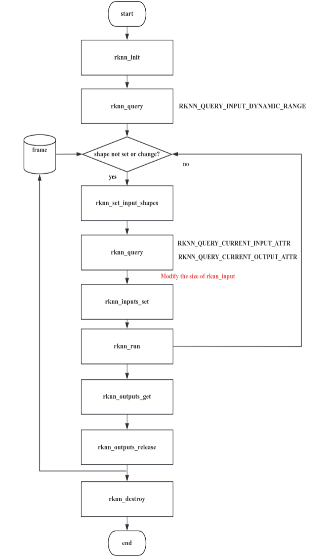
Figure 5-11 Zero-copy API calling process of dynamic shape input interface
Initialization, query the input shape list supported by the RKNN model, and set the input shape are the same as the above general API, therefore will not be described here. The difference is that the interface used after setting the input shape. An example of zero-copy inference C code is as follows:
// Create the largest input tensor memory
rknn_tensor_mem *input_mems[io_num.n_input];
for (int i = 0; i < io_num.n_input; i++) {
  // default input type is int8 (normalize and quantize need compute in outside)
  // if set uint8, will fuse normalize and quantize to npu
  input_attrs[i].type = RKNN_TENSOR_UINT8;
  // default fmt is NHWC, npu only support NHWC in zero copy mode
  input_attrs[i].fmt = RKNN_TENSOR_NHWC;
  input_mems[i] = rknn_create_mem(ctx, input_attrs[i].size_with_stride);
...
// Create the largest output tensor memory
rknn_tensor_mem *output_mems[io_num.n_output];
for (uint32_t i = 0; i < io_num.n_output; ++i) {
  // default output type is depend on model, this require float32 to compute top5
  // allocate float32 output tensor
  int output_size = output_attrs[i].size * sizeof(float);
  output_mems[i] = rknn_create_mem(ctx, output_size);
...
// Load the input and set the model input shape. This is called once each time the input shape is switched.
for (int s = 0; s < shape_num; ++s) {
  for (int i = 0; i < io_num.n_input; i++) {
    for (int j = 0; j < input_attrs[i].n_dims; ++j) {
      input_attrs[i].dims[j] = shape_range[i].dyn_range[s][j];
  ....
  ret = rknn_set_input_shapes(ctx, io_num.n_input, input_attrs);
  if (ret < 0) {
    fprintf(stderr, "rknn_set_input_shape error! ret=%d\n", ret);
    return -1;
  ...
  // Get the input and output shape of the current inference
  printf("current input tensors:\n");
  rknn_tensor_attr cur_input_attrs[io_num.n_input];
  memset(cur_input_attrs, 0, io_num.n_input * sizeof(rknn_tensor_attr));
  for (uint32_t i = 0; i < io_num.n_input; i++) {
    cur_input_attrs[i].index = i;
    // query info
    ret = rknn_query(ctx, RKNN_QUERY_CURRENT_INPUT_ATTR, &(cur_input_attrs[i]), sizeof(rknn_tensor_attr));

    if (ret < 0) {
      printf("rknn_init error! ret=%d\n", ret);
      return -1;
  dump_tensor_attr(&cur_input_attrs[i]);
  ...
  printf("current output tensors:\n");
  rknn_tensor_attr cur_output_attrs[io_num.n_output];
  memset(cur_output_attrs, 0, io_num.n_output * sizeof(rknn_tensor_attr));
  for (uint32_t i = 0; i < io_num.n_output; i++) {
    cur_output_attrs[i].index = i;
    // query info
    ret = rknn_query(ctx, RKNN_QUERY_CURRENT_OUTPUT_ATTR, &(cur_output_attrs[i]),
sizeof(rknn_tensor_attr));
     if (ret != RKNN_SUCC) {
       printf("rknn_query fail! ret=%d\n", ret);
       return -1;
   dump_tensor_attr(&cur_output_attrs[i]);
   ...
   // Specify the number of NPU cores, only 3588/3576 is supported
   rknn_set_core_mask(ctx, (rknn_core_mask)core_mask);

   // Set input information
   rknn_input inputs[io_num.n_input];
   memset(inputs, 0, io_num.n_input * sizeof(rknn_input));
   std::vector<cv::Mat> resize_imgs;
   resize_imgs.resize(io_num.n_input);
   for (int i = 0; i < io_num.n_input; i++) {
     int height = cur_input_attrs[i].fmt == RKNN_TENSOR_NHWC ? cur_input_attrs[i].dims[1] :
 cur_input_attrs[i].dims[2];
     int width = cur_input_attrs[i].fmt == RKNN_TENSOR_NHWC ? cur_input_attrs[i].dims[2] :
 cur_input_attrs[i].dims[3];
     int stride = cur_input_attrs[i].w_stride;
     cv::resize(imgs[i], resize_imgs[i], cv::Size(width, height));
     int input_size = resize_imgs[i].total() * resize_imgs[i].channels();
     // Copy external data to zero-copy input buffer
     if (width == stride)
       memcpy(input_mems[i]->virt_addr, resize_imgs[i].data, input_size);
     else {
       int height = cur_input_attrs[i].dims[1];
       int channel = cur_input_attrs[i].dims[3];
       // copy from src to dst with stride
       uint8_t *src_ptr = resize_imgs[i].data;
       uint8_t *dst_ptr = (uint8_t *)input_mems[i]->virt_addr;
       // width-channel elements
       int src_wc_elems = width * channel;
       int dst_wc_elems = stride * channel;
       for (int b = 0; b < cur_input_attrs[i].dims[0]; b++) {
         for (int h = 0; h < height; ++h) {
           memcpy(dst_ptr, src_ptr, src_wc_elems);
           src_ptr += src_wc_elems;
           dst_ptr += dst_wc_elems;
    ....
   // Update input zero-copy buffer
   for (int i = 0; i < io_num.n_input; i++) {
     cur_input_attrs[i].type = RKNN_TENSOR_UINT8;
     ret = rknn_set_io_mem(ctx, input_mems[i], &cur_input_attrs[i]);
     if (ret < 0) {
       printf("rknn_set_io_mem fail! ret=%d\n", ret);
       return -1;
   ....
   // Update output zero-copy buffer
   for (uint32_t i = 0; i < io_num.n_output; ++i) {
     // default output type is depend on model, this require float32 to compute top5
     cur_output_attrs[i].type = RKNN_TENSOR_FLOAT32;
     cur_output_attrs[i].fmt = RKNN_TENSOR_NCHW;
     // set output memory and attribute
     ret = rknn_set_io_mem(ctx, output_mems[i], &cur_output_attrs[i]);
     if (ret < 0) {
       printf("rknn_set_io_mem fail! ret=%d\n", ret);
      return -1;
  ....
  // Inference
  printf("Begin perf ...\n");
  double total_time = 0;
  for (int i = 0; i < loop_count; ++i) {
    int64_t start_us = getCurrentTimeUs();
    ret = rknn_run(ctx, NULL);
    int64_t elapse_us = getCurrentTimeUs() - start_us;
    if (ret < 0) {
      printf("rknn run error %d\n", ret);
      return -1;
    ...
    total_time += elapse_us / 1000.f;
    printf("%4d: Elapse Time = %.2fms, FPS = %.2f\n", i, elapse_us / 1000.f, 1000.f * 1000.f / elapse_us);
  ...
  printf("Avg FPS = %.3f\n", loop_count * 1000.f / total_time);
Note:
1. The rknn_set_io_mem() interface in the case of dynamic shape, the shape and size description of the input buffer:
After initialization is completed and before calling the rknn_set_input_shapes() interface, the rknn_query() interface uses RKNN_QUERY_INPUT_ATTR and RKNN_QUERY_OUTPUT_ATTR to query the shape of input and output tensor is usually the largest size. Users can use the sizes obtained by these two commands to allocate input and output memory. If there is a multi-input model, the shape of some inputs may not be the largest. In this case, you need to search for the largest size among the supported shapes and allocate the largest input and output memory.
If the input is non-4-dimensional, use fmt=UNDEFINED, pass the buffer size of the original model input shape is calculated based on the input shape and type.
If the input is 4 dimensions, fmt=NHWC or NC1HWC2 is supported, the corresponding fields through rknn_query to obtain the shape and size are passing to the NHWC or NC1HWC2 shape and corresponding size buffer.
In the rknn_query() interface, when the flags are RKNN_QUERY_CURRENT_INPUT_ATTR and RKNN_QUERY_CURRENT_OUTPUT_ATTR, the input/output shape of the original model is obtained and the format is NHWC or UNDEFINED; when the flags are RKNN_QUERY_CURRENT_NATIVE_INPUT_ATTR and RKNN_QUERY_CURRENT_NATIVE_OUTPUT_ATTR, get model input/output with optimal performance for NPU and the format is NHWC or NC1HWC2.
2. When the buffer arrangement format used in the rknn_set_io_mem() interface is NHWC, the shape and fmt in rknn_tensor_attr need to be set according to the information queried by RKNN_QUERY_CURRENT_INPUT_ATTR. If the buffer arrangement format used is NC1HWC2, the shape and fmt in rknn_tensor_attr need to be set according to the information queried by RKNN_QUERY_CURRENT_NATIVE_INPUT_ATTR.
For the complete dynamic shape C API Demo, please refer to (https://github.com/airockchip/rknn-toolkit2/tree/ma ster/rknpu2/examples/rknn_dynamic_shape_input_demo)
5.5 Custom Operators
5.5.1 Introduction
RKNN SDK provides a mechanism for custom operators, which allows developers to define and execute custom operators in the inference of the RKNN model. By implementing custom operators, developers can extend and optimize model functions for specific hardware (CPU or GPU) to make full use of hardware resources and increase inference speed. At the same time, developing custom operators requires a deep understanding of deep learning computing principles and the characteristics of the target hardware platform to ensure correctness and performance. Currently only ONNX model custom operators are supported.
RKNN custom operators mainly include two major steps:
Use RKNN-Toolkit2 to register custom operators and export RKNN models.
Write the C code implementation of the custom operator, load, register and execute it through the RKNN API.
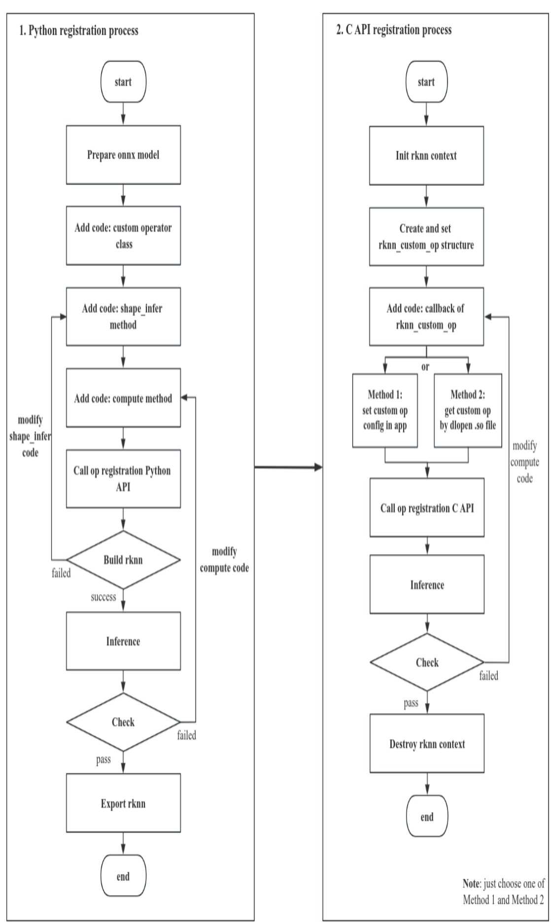
Figure 5-12 Complete process of registering custom operators
5.5.2 Overall Process
5.5.2.1 Use RKNN-Toolkit2 to register custom operators and export RKNN models
1. Prepare the onnx model: According to the ONNX specification, the user designs the op type, name, attributes, input/output number of the custom operator, and inserts the operator into the topology graph position in onnx. The user designs and exports onnx models using the API provided by the onnx package.
2. Implement the custom operator Python class, which mainly includes two function interfaces: shape_infer() and compute(), and call rknn.reg_custom_op() to register the operator.
3. If rknn.build() is executed successfully, inference can be performed, otherwise you need to check the shape_infer() code implementation in step 2. Then run the simulation. If the simulation results are correct, you can call the rknn.export_rknn() interface to export the RKNN model. Otherwise, you need to check the compute() code in step 2.
5.5.2.2 C code implementation of the custom operator, load, register and execute through RKNN API.
1. Based on the rknn_custom_op class of rknn_custom_op.h, write the C code implementation of the custom operator. After the writing is completed, fill in the information of the rknn_custom_op class.
2. Call rknn_register_custom_ops() to register the information of the rknn_custom_op class.
3. Refer to the process of the general API or zero-copy API to build and infer the model. You can turn on the model detailed log and dump function to confirm the correctness of the custom operator implementation.
5.5.2.3 Use RKNN-Toolkit2 device connected inference or accuracy analysis
If the user needs to perform device connected accuracy analysis on a model containing a custom operator, need to compile the callback function implementation code of the custom operator into .so, place it in the specified path, and restart rknn_server. Please refer to Chapter 5.5.4.4 for details.
5.5.3 Python Process
Currently, only the onnx model supports custom operators, allowing users to add Non-ONNX standard operators supported by RKNN.
Adding an Non-ONNX standard custom operator is used to add a new operator that does not exist in the ONNX operator list. In addition to meeting the ONNX spec specification, the operator must also meet the following rules:
The op_type of the operator cannot be the same as the ONNX standard operator. It is recommended to start with the “cst” character.
The operator must have a connection relationship with other operators, including the shape of each input/output, data type, etc.
Operator input attributes support single values or arrays of types bool, int32, float32, and int64.
Operator constant input supports bool, int32, float32, and int64 types. This type refers to the data type of the unquantized ONNX model.
Because the Non-ONNX standard operator is not a standard operator in the ONNX SPEC. Therefore, users need to build and export an ONNX model containing the Non-ONNX standard operator through the ONNX API or the API of other frameworks.
For convenience, a simple modification of the definition of Softmax is used as an example to build an ONNX model containing the Non-ONNX standard operator cstSoftmax. The modification method is as follows:
import onnx

path="test_softmax.onnx"
model=onnx.load(path)

for node in model.graph.node:
  if node.op_type =="Softmax":
    node.op_type = "cstSoftmax"
    ... # Modify the attribute definition of cstSoftmax, etc
onnx.save(model, "./test_softmax_custom.onnx")
After building an onnx model containing custom operators, you can use Netron to open the ONNX model and check whether the custom operator meets the specifications. Then you can implement the custom operator class, as follows (taking custom Softmax as an example):
import numpy as np
from rknn.api.custom_op import get_node_attr
class cstSoftmax:
  op_type = 'cstSoftmax'
  def shape_infer(self, node, in_shapes, in_dtypes):
    out_shapes = in_shapes.copy()
    out_dtypes = in_dtypes.copy()
    return out_shapes, out_dtypes
  def compute(self, node, inputs):
    x = inputs[0]
    axis = get_node_attr(node, 'axis')
    x_max = np.max(x, axis=axis, keepdims=True)
    tmp = np.exp(x - x_max)
    s = np.sum(tmp, axis=axis, keepdims=True)
    outputs = [tmp / s]
    return outputs
The custom operator must be a Python class.
The custom operator class must contain a string variable named op_type, which is consistent with the name of the custom operator type in the ONNX.
The custom operator class must contain the member function shape_infer(self, node, in_shapes, in_dtypes). The function name and parameter name must be consistent, otherwise an error will be reported. This function is used for shape inference of custom operators. Among node is the operator node object of ONNX, which contains the attributes and input and output information of the custom operator; in_shapes is the shape information of all inputs of the operator, the format is [shape_0, shape_1, …], and the type of the shape in the list is a list; in_dtypes is the dtype information of all inputs to the operator, the format is [dtype_0, dtype_1, …], and the type of the dtype in the list is the numpy’s dtype. In addition, this function needs to return all the output shape information and dtype information of the operator, and the format is consistent with in_shapes and in_dtypes.
The custom operator class must contain the member function compute(self, node, inputs), and the function name and parameter name must be consistent, otherwise an error will be reported. This function is used for inference of custom operators. Among node is the operator node object of ONNX, which contains the attributes and input and output information of the custom operator; inputs is the input data of the operator, and the format is [array_0, array_1, …], and the type of the dtype in the list is the numpy’s ndarray. In addition, this function needs to return all output data of the operator, in the same format as inputs.
If the custom operator contains custom attributes, you can obtain the attribute value of the custom operator through from rknn.api.custom_op import get_node_attr.
After completing the custom operator class, you can register the operator class through rknn.reg_custom_op(). After registration, you can call rknn.build() to convert and generate the RKNN model. Custom operator classes can ensure normal functions such as model conversion and inference. The specific implementation is as follows (taking custom Softmax as an example):
from rknn.api import RKNN
# Create RKNN object
rknn = RKNN(verbose=True)

# Pre-process config
print('--> Config model')
rknn.config(mean_values=[103.94, 116.78, 123.68], std_values=[58.82, 58.82, 58.82], quant_img_RGB2BGR=True,
target_platform='rk3566')
print('done')

print('--> Register cstSoftmax op')
ret = rknn.reg_custom_op(cstSoftmax())
if ret != 0:
  print('Register cstSoftmax op failed!')
  exit(ret)
print('done')

print('--> Loading model')
ret = rknn.load_onnx(model='mobilenet_v2.onnx')
if ret != 0:
  print('Load model failed!')
  exit(ret)
print('done')

# Build model
print('--> Building model')
ret = rknn.build(do_quantization=True, dataset='./dataset.txt')
if ret != 0:
  print('Build model failed!')
  exit(ret)
print('done')
rknn.reg_custom_op() needs to be called between rknn.config() and rknn.load_xxx().
5.5.4 C API Deployment
After obtaining the RKNN model with custom operators, start calling the C API for deployment. First, the structure and interface of the custom operators are located in the rknn_custom_op.h, and the developer program needs to include this head file. The process of using custom operators is shown in the figure below:
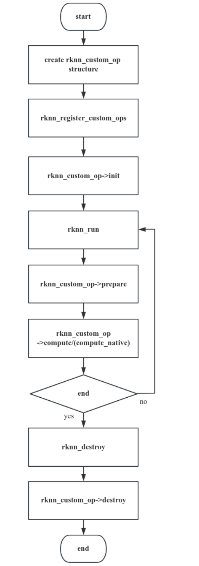
Figure 5-13 C API calling process for registering custom operators
5.5.4.1 Initialize Custom Operator Structure
After creating the rknn context, developers need to create the rknn_custom_op structure and set custom operator information. Operator information includes the following:
version: The version of the operator.
target: The execution backend of the operator, currently supports CPU and GPU.
op_type: The type of operator, which is the same as the type in the ONNX model.
cl_kernel_name: cl_kernel function name of OpenCL code. Must be configured when registering a GPU operator.
cl_kernel_source: The full path of the .cl file of the custom operator or the OpenCL kernel string. When cl_source_size=0, it represents the full path of the .cl file; when cl_source_size>0, it represents the OpenCL kernel code string. Must be configured when registering a GPU operator.
cl_source_size: The size of cl_kernel_source. Size equal to 0 is a special case, it means cl_kernel_source is the path.
cl_build_options: OpenCL kernel compilation options, passed in as a string. Must be configured when registering a GPU operator.
init: optional, called once in rknn_register_custom_ops.
prepare: optional, it is a preprocessing callback function. Each time rknn_run will execute prepare and compute/compute_native callback functions, the order of execution is prepare first, compute/compute_native last.
compute: Must be implemented, operator computation callback function, its input/output are NCHW float32 format data (onnx model if the input/output is int64 data type, it will be int64 format data)
compute_native: reserved, please set to NULL.
destroy: optional, executed once in rknn_destory.
The init/prepare/compute callback function parameter definition specifications are as follows:
rknn_custom_op_context* op_ctx: context information of op callback function
rknn_custom_op_tensor* inputs: op input tensor data and information
uint32_t n_inputs: number of op inputs
rknn_custom_op_tensor* outputs: op output tensor data and information
uint32_t n_outputs: number of op outputs
The destroy callback function only has one parameter: rknn_custom_op_context* op_ctx.
rknn_custom_op_context
Contains target (execution backend device), GPU context, custom operator private context and priv_data, of which priv_data is managed by the developer (assignment, reading, writing, and destroy). The GPU context includes cl_context, cl_command_queue, and cl_kernel pointers, which can be passed forced type conversion to obtain the corresponding OpenCL object.
priv_data is a pointer that the user can choose to configure or not. The usual usage is that the user creates a resource in the init() callback function, points priv_data to the memory address and applys in the prepare()/compute() callback function, finally in destroy resources within the destroy() callback function.
rknn_custom_op_tensor
Represents input/output tensor information, including tensor name, shape, size, quantization parameters, virtual base address, fd, data offset and other information.
The user does not need to create the input and output Tensor memory of the operator in the callback compute() callback function. The data corresponding to the virtual address is ready when entering the compute() callback function. The calculation formula of virtual address is Tensor’s effective address = virtual base address + data offset. The virt_addr of the mem member represents the virtual base address, and the offset of the mem member represents the data offset (in bytes). The user can read the effective address of the input tensor in the callback function, which points to the output data calculated by the previous layer operator, and the effective address of the output tensor points for the input that will be sent to the next layer operator.
rknn_custom_op_attr
The developer obtains the attribute information by calling the rknn_custom_op_get_op_attr() interface and passing in the attribute field. The attribute information is represented by rknn_custom_op_attr. The void type buffer, dtype and number of elements in rknn_custom_op_attr represent a memory segment. The developers can obtain an array of the corresponding numerical type by forcefully casting the buffer pointer type in C/C++ based on the dtype.
5.5.4.1.1 Init Callback Function
It is used for parsing operator information or initializing temporary buffers or input/output buffers, such as for allocating a temporary buffer. The sample code of the init callback function is as follows:
CPU Operator:
/**
* cpu kernel init callback for custom op
*/
int custom_op_init_callback(rknn_custom_op_context* op_ctx, rknn_custom_op_tensor* inputs, uint32_t n_inputs,
              rknn_custom_op_tensor* outputs, uint32_t n_outputs)
{
  printf("custom_op_init_callback\n");
  // create tmp buffer
  float* tmp_buffer = (float*)malloc(inputs[0].attr.n_elems * sizeof(float));
  op_ctx->priv_data = tmp_buffer;
  return 0;
}
GPU Operator:
/**
* opencl kernel init callback for custom op
* */
int relu_init_callback_gpu(rknn_custom_op_context* op_ctx, rknn_custom_op_tensor* inputs, uint32_t n_inputs,
             rknn_custom_op_tensor* outputs, uint32_t n_outputs)
{
  printf("relu_init_callback_gpu\n");
  // 获取opencl context
  cl_context cl_ctx = (cl_context)op_ctx->gpu_ctx.cl_context;

  // create tmp cl buffer
  cl_mem* memObject = (cl_mem*)malloc(sizeof(cl_mem) * 2);
  memObject[0] = clCreateBuffer(cl_ctx, CL_MEM_READ_WRITE, inputs[0].attr.size, NULL, NULL);
  memObject[1] = clCreateBuffer(cl_ctx, CL_MEM_READ_WRITE, outputs[0].attr.size, NULL, NULL);
  op_ctx->priv_data = memObject;
  return 0;
}
5.5.4.1.2 Prepare Callback Function
This callback function is called for each frame inference and is currently reserved for future.
5.5.4.1.3 Compute Callback Function
It is the computation function for a custom operator, and developers must complete the core function for input/output with NCHW or UNDEFINED format and float32 data type.
1. Compute callback(CPU)
Assuming performs the softmax function, the CPU operator’s compute function as an example below:
/**
* float32 kernel implemetation sample for custom op
* */
int compute_custom_softmax_float32(rknn_custom_op_context* op_ctx, rknn_custom_op_tensor* inputs, uint32_t
n_inputs,
                 rknn_custom_op_tensor* outputs, uint32_t n_outputs)
{
  unsigned char* in_ptr = (unsigned char*)inputs[0].mem.virt_addr + inputs[0].mem.offset;
  unsigned char* out_ptr = (unsigned char*)outputs[0].mem.virt_addr + outputs[0].mem.offset;
  int axis = 0;
  const float* in_data = (const float*)in_ptr;
  float* out_data = (float*)out_ptr;
  std::string name = "";
  rknn_custom_op_attr op_name;
  rknn_custom_op_get_op_attr(op_ctx, "name", &op_name);
  if (op_name.n_elems > 0 && op_name.dtype == RKNN_TENSOR_UINT8) {
    name = (char*)op_name.data;
  }

  rknn_custom_op_attr op_attr;
  rknn_custom_op_get_op_attr(op_ctx, "axis", &op_attr);
  if (op_attr.n_elems == 1 && op_attr.dtype == RKNN_TENSOR_INT64) {
    axis = ((int64_t*)op_attr.data)[0];
  }

  printf("op name = %s, axis = %d\n", name.c_str(), axis);
  float* tmp_buffer = (float*)op_ctx->priv_data;
  // kernel implemetation for custom op
  {
    int inside = 1;
    int outside = 1;
    int channel = 1;

    while (axis < 0) {
      axis += inputs[0].attr.n_dims;
    }

    for (int i = 0; i < axis; i++) {
      outside *= inputs[0].attr.dims[i];
    }
    channel = inputs[0].attr.dims[axis];
    for (int i = axis; i < inputs[0].attr.n_dims; i++) {
      inside *= inputs[0].attr.dims[i];
    }
    for (int y = 0; y < outside; y++) {
      const float* src_y = in_data + y * inside;
      float* dst_y = out_data + y * inside;
      float max_data = -FLT_MAX;
      float sum_data = 0.0f;

      for (int i = 0; i < inside; ++i) {
        max_data = fmaxf(max_data, src_y[i]);
      }
      for (int i = 0; i < inside; ++i) {
        tmp_buffer[i] = expf(src_y[i] - max_data);
        sum_data += tmp_buffer[i];
      }
      for (int i = 0; i < inside; ++i) {
        dst_y[i] = tmp_buffer[i] / sum_data;
      }
    }
  }
  return 0;
}
2. Compute callback(GPU)
For GPU operators, developers can complete the following steps in the callback function:
Developers can retrieve the cl_context, cl_command_queue, and cl_kernel objects from the gpu_ctx in the rknn_custom_op_context. This process requires developers to perform data type conversions.
If necessary, cl_mem object buffer of op input or output created by the user.
Set the function arguments of the cl_kernel.
The input buffer data for the OpenCL kernel currently only supports the float data type; other types are not supported.
In the case of zero-copy usage, developers can use clImportMemoryARM to assist in mapping the memory of the input tensor to the cl_mem structure in OpenCL. The input tensor already contains the input data, so developers do not need to copy it again. This process can also be handled in the init callback function, and then the cl_mem structure can be recorded in the priv_data member. Finally, retrieve and use the priv_data in the compute callback.
Execute the cl_kernel in a blocking manner.
The input data within the CL kernel is provided in the NCHW format.
If the developer needs the CPU to access data after the GPU operation is completed, the developer needs to refresh the cache of the output Tensor by calling the rknn_mem_sync function before reading the data.
Assume that the developer wants to implement a custom layer to complete the relu function. Examples of GPU operator calculation functions are as follows:
/**
* opencl kernel init callback for custom op
* */
int compute_custom_relu_float32(rknn_custom_op_context* op_ctx, rknn_custom_op_tensor* inputs, uint32_t
num_inputs,
                rknn_custom_op_tensor* outputs, uint32_t num_outputs)
{
   std::string name = "";
   rknn_custom_op_attr op_name;
   rknn_custom_op_get_op_attr(op_ctx, "name", &op_name);
   if (op_name.n_elems > 0 && op_name.dtype == RKNN_TENSOR_UINT8) {
     name = (char*)op_name.data;
   }

   // // save input npy
   // char output_path[PATH_MAX];
   // sprintf(output_path, "%s/cpu_input%d.npy", ".", 0);
   // save_npy(output_path, (float*)in_data, &inputs[0].attr);

   // get context
   cl_context cl_ctx = (cl_context)op_ctx->gpu_ctx.cl_context;

   // get command queue
   cl_command_queue queue = (cl_command_queue)op_ctx->gpu_ctx.cl_command_queue;

   // get kernel
   cl_kernel kernel = (cl_kernel)op_ctx->gpu_ctx.cl_kernel;

   // import input/output buffer
   const cl_import_properties_arm props[3] = {
     CL_IMPORT_TYPE_ARM,
     CL_IMPORT_TYPE_DMA_BUF_ARM,
     0,
   };

   cl_int status;
   cl_mem inObject = clImportMemoryARM(cl_ctx, CL_MEM_READ_WRITE, props, &inputs[0].mem.fd,
                     inputs[0].mem.offset + inputs[0].mem.size, &status);
   if (status != CL_SUCCESS) {
     printf("Tensor: %s clImportMemoryARM failed\n", inputs[0].attr.name);
   }
   cl_mem outObject = clImportMemoryARM(cl_ctx, CL_MEM_READ_WRITE, props, &outputs[0].mem.fd,
                     outputs[0].mem.offset + outputs[0].mem.size, &status);
   if (status != CL_SUCCESS) {
     printf("Tensor: %s clImportMemoryARM failed\n", outputs[0].attr.name);
   }

   int in_type_bytes = get_type_bytes(inputs[0].attr.type);
   int out_type_bytes = get_type_bytes(outputs[0].attr.type);
   int in_offset = inputs[0].mem.offset / in_type_bytes;
   int out_offset = outputs[0].mem.offset / out_type_bytes;
   unsigned int elems = inputs[0].attr.n_elems;

   // set kernel args
   int argIndex = 0;
   clSetKernelArg(kernel, argIndex++, sizeof(cl_mem), &inObject);
   clSetKernelArg(kernel, argIndex++, sizeof(cl_mem), &outObject);
   clSetKernelArg(kernel, argIndex++, sizeof(int), &in_offset);
   clSetKernelArg(kernel, argIndex++, sizeof(int), &out_offset);
   clSetKernelArg(kernel, argIndex++, sizeof(unsigned int), &elems);

   // set global worksize
   const size_t global_work_size[3] = {elems, 1, 1};
  // enqueueNDRangeKernel
  clEnqueueNDRangeKernel(queue, kernel, 1, NULL, global_work_size, NULL, 0, NULL, NULL);

  // finish command queue
  clFinish(queue);

  // //cpu access data after sync to device
  // rknn_mem_sync(&outputs[0].mem, RKNN_MEMORY_SYNC_FROM_DEVICE);
  // // save output npy
  // char output_path[PATH_MAX];
  // sprintf(output_path, "%s/cpu_output%d.npy", ".", 0);
  // unsigned char* out_data = (unsigned char*)outputs[0].mem.virt_addr+outputs[0].mem.offset;
  // save_npy(output_path, (float*)out_data, &inputs[0].attr);
  return 0;
}
5.5.4.1.4 Destroy Callback Function
It is used to destroy temporary buffers or input/output buffers of custom operators. The sample code to destroy the temporary buffer is as follows:
CPU Operator
/**
* cpu kernel destroy callback for custom op
*/
int custom_op_destroy_callback(rknn_custom_op_context* op_ctx)
{
  printf("custom_op_destroy_callback\n");
  // clear tmp buffer
  free(op_ctx->priv_data);
  return 0;
}
GPU Operator
/**
* opencl kernel destroy callback for custom op
*/
int relu_destroy_callback_gpu(rknn_custom_op_context* op_ctx)
{
  // clear tmp buffer
  printf("relu_destroy_callback_gpu\n");
  cl_mem* memObject = (cl_mem*)op_ctx->priv_data;
  clReleaseMemObject(memObject[0]);
  clReleaseMemObject(memObject[1]);
  free(memObject);
  return 0;
}
5.5.4.2 Register Custom Operator
After setting the rknn_custom_op structure, you need to call rknn_register_custom_ops() to register it in rknn_context. This interface supports registering multiple custom operators at the same time.
After completing the CPU’s compute callback function, the code example for registering a CPU custom operator named “cstSoftmax” and “ArgMax” is as follows:
CPU Operator
// CPU operators
rknn_custom_op user_op[2];
memset(user_op, 0, 2 * sizeof(rknn_custom_op));
strncpy(user_op[0].op_type, "cstSoftmax", RKNN_MAX_NAME_LEN - 1);
user_op[0].version = 1;
user_op[0].target = RKNN_TARGET_TYPE_CPU;
user_op[0].init = custom_op_init_callback;
user_op[0].compute = compute_custom_softmax_float32;
user_op[0].destroy = custom_op_destroy_callback;

strncpy(user_op[1].op_type, "ArgMax", RKNN_MAX_NAME_LEN - 1);
user_op[1].version = 1;
user_op[1].target = RKNN_TARGET_TYPE_CPU;
user_op[1].init = custom_op_init_callback;
user_op[1].compute = compute_custom_argmax_float32;
user_op[1].destroy = custom_op_destroy_callback;

ret = rknn_register_custom_ops(ctx, user_op, 2);
if (ret < 0) {
  printf("rknn_register_custom_ops fail! ret = %d\n", ret);
  return -1;
}
GPU Operator
For GPU operators, OpenCL kernel registration is supported in two ways: constant string or file path. When cl_source_size in the rknn_custom_op structure is equal to 0, cl_kernel_source represents the file path of the OpenCL kernel. When cl_source_size is greater than 0, cl_kernel_source represents the OpenCL kernel function string. The sample code of the OpenCL kernel with relu function saved as a string is as follows:
char* cl_kernel_source = "#pragma OPENCL EXTENSION cl_arm_printf : enable"
  "#pragma OPENCL EXTENSION cl_khr_fp16 : enable "
  " __kernel void relu_float(__global const float* input, __global float* output, int "
  "in_offset, int out_offset, const unsigned int elems) "
  "{"
  " int gid = get_global_id(0);"
  " if (gid < elems) {"
  " float in_value = input[in_offset + gid];"
  " output[out_offset + gid] = in_value >= 0.f ? in_value : 0.f;"
  " }"
  "}"
  "__kernel void relu_half(__global const half* input, __global half* output, int in_offset, "
  "int out_offset, const unsigned int elems)"
  "{"
  " int gid = get_global_id(0);"
  " if (gid < elems) {"
  " half in_value = input[in_offset + gid];"
  " output[out_offset + gid] = in_value >= 0.f ? in_value : 0.f;"
  " }"
  "}";
After completing the OpenCL kernel function and the GPU compute callback function, you can set the rknn_custom_op structure array and register the GPU operator. The sample code for registering the GPU operator is as follows:
// GPU operators
rknn_custom_op user_op[1];
memset(user_op, 0, sizeof(rknn_custom_op));
strncpy(user_op->op_type, "cstSoftmax", RKNN_MAX_NAME_LEN - 1);
user_op->version = 1;
user_op->target = RKNN_TARGET_TYPE_GPU;
user_op->init = relu_init_callback_gpu;
user_op->compute = compute_custom_relu_float32;
user_op->destroy = relu_destroy_callback_gpu;
#ifdef LOAD_FROM_PATH
user_op->cl_kernel_source = "./custom_op.cl";
user_op->cl_source_size = 0;
#else
user_op->cl_kernel_source = cl_kernel_source;
user_op->cl_source_size = strlen(cl_kernel_source);
#endif
strcpy(user_op->cl_kernel_name, "relu_float");

ret = rknn_register_custom_ops(ctx, user_op, 1);
if (ret < 0) {
  printf("rknn_register_custom_ops fail! ret = %d\n", ret);
  return -1;
}
Before registering and calling this interface, you must clearly define the op_type of the custom operator, prepare the operator information and configure the rknn_custom_op array. Each type of custom operator must call the registration interface once, and operators of the same type on the network must be called only once.
5.5.4.3 Model Inference
After registering all operators, you can use the general API or zero-copy API process to complete inference.
5.5.4.4 Connected Device Accuracy Analysis
The board-connected debugging function of custom operators requires that the rknn_server version >= 1.6.0.
During connected debugging, rknn_server will use dlopen to open the user-compiled custom operator plugin library from a specific directory to obtain operator information. For registration of custom operators in the plugin library, the user must implement a function called get_rknn_custom_op( ).
If the user needs to perform connected device accuracy analysis on a model containing custom operators, the specific steps are as follows:
1. Implement a get_rknn_custom_op() function and the necessary callback function, and compile it into a library corresponding to the system. The compiled plugin library name must be prefixed with “librkcst_”, for example, the library name is librkcst_relu.so.
2. Place the plugin in /vendor/lib64/ (Android arm64-v8a) or /usr/lib/rknpu/op_plugins (Linux)
3. Use the Python interface of RKNN-Toolkit2 on the computer to perform connected device accuracy analysis.
The sample code of get_rknn_custom_op function is as follows:
/**
 * To obtain operator information to be registered, a plugin library must have one and only one of this function.
 */
RKNN_CUSTOM_OP_EXPORT rknn_custom_op* get_rknn_custom_op()
{
  // register a custom op
  memset(&user_op, 0, sizeof(rknn_custom_op));
  strncpy(user_op.op_type, "cstSoftmax", RKNN_MAX_NAME_LEN - 1);
  user_op.version = 1;
  user_op.target = RKNN_TARGET_TYPE_CPU;
  user_op.init = custom_op_init_callback;
  user_op.compute = compute_custom_softmax_float32;
  user_op.destroy = custom_op_destroy_callback;
  return &user_op;
}
The get_rknn_custom_op function must add the RKNN_CUSTOM_OP_EXPORT attribute to let the plugin export the get_rknn_custom_op function symbol.
rknn_server calls dlopen to obtain all so library file handles in a specific directory, and then uses the dlsym function to obtain the get_rknn_custom_op function pointer. The custom operator structure can be obtained by calling the function pointer. The sample code is as follows:
std::vector<std::string> get_all_plugin_paths(std::string plugin_dir)
{
  std::vector<std::string> plugin_paths;
  if (access(plugin_dir.c_str(), 0) != 0) {
    fprintf(stderr, "Can not access plugin directory: %s, please check it!\n", plugin_dir.c_str());
  }

  DIR* dir;
  struct dirent* ent;
  const char* prefix = RKNN_CSTOP_PLUGIN_PREFIX; // All library file names should start with this prefix

  if ((dir = opendir(plugin_dir.c_str())) != NULL) {
    while ((ent = readdir(dir)) != NULL) {
      if (ent->d_type == DT_REG) {
        const char* filename = ent->d_name;
        size_t len = strlen(filename);

        if (len > 10 && strncmp(filename, prefix, strlen(prefix)) == 0) {
          printf("Found plugin: %s file in %s\n", filename, plugin_dir.c_str());
          plugin_paths.push_back(plugin_dir + "/" + filename);
        }
      }
    }
    closedir(dir);
  } else {
    fprintf(stderr, "Unable to open directory");
  }
  return plugin_paths;
}

// the default path of the custom operator plugin libraries
std::string plugin_dir =
#if defined(__ANDROID__)
# if defined(__aarch64__)
  "/vendor/lib64/";
# else
  "/vendor/lib/";
# endif // __aarch64__
#elif defined(__linux__)
  "/usr/lib/rknpu/op_plugins/";
#endif

std::vector<std::string> plugin_paths = get_all_plugin_paths(plugin_dir);
std::vector<void*> so_handles;
for (auto path : plugin_paths) {
  printf("load plugin %s\n", path.c_str());
  void* plugin_lib = dlopen(path.c_str(), RTLD_NOW);
  char* error = dlerror();
  if (error != NULL) {
    fprintf(stderr, "dlopen %s fail: %s.\nPlease try to set 'export LD_LIBRARY_PATH=$LD_LIBRARY_PATH:%s'\n",
        path.c_str(), error, plugin_dir.c_str());
    dlclose(plugin_lib);
    return -1;
  }
  printf("dlopen %s successfully!\n", path.c_str());
  get_custom_op_func custom_op_func = (get_custom_op_func)dlsym(plugin_lib, "get_rknn_custom_op");
  error = dlerror();
  if (error != NULL) {
    fprintf(stderr, "dlsym fail: %s\n", error);
    dlclose(plugin_lib);
    return -1;
  }

  rknn_custom_op* user_op = custom_op_func();
  ret = rknn_register_custom_ops(ctx, user_op, 1);
  if (ret < 0) {
    printf("rknn_register_custom_ops fail! ret = %d\n", ret);
    return -1;
  }
  so_handles.push_back(plugin_lib);
}
The plugin library has the following notices:
A custom operator plugin library can only register one custom operator. If you need to register multiple custom operators, you need to create multiple plugin libraries.
The name of the plugin library must start with “librkcst_” and end with .so.
If it is a plugin library implemented in C++ code, in order to correctly open the function symbols in the C interface, the following macros must be added before and after the function definition:
#ifdef __cplusplus
extern "C" {
#endif

//code

#ifdef __cplusplus
} // extern "C"
#endif
If the dlopen fails to load the plugin library, it is necessary to check if the LD_LIBRARY_PATH environment variable is set and verify that the directory containing the plugin library is included in the specified path.
5.6 Multi-Batch Instruction
5.6.1 Multi-Batch Principle
There are three cores inside the RK3588 NPU and two cores inside the RK3576 NPU. In order to make multi- batch inference more efficient, a multi-batch inference method is provided. When multiple batches are enabled, rknn_dup_context will be called internally to copy the context (rknn_dup_context will only copy the Internal of the context, and the Weight will be reused). Copy once when rknn_batch_size=2, and copy twice when rknn_batch_size >=3 (there are only 3 cores working at the same time, and only copy twice to avoid memory waste). Each context core_mask will be set to 0 to allow automatic scheduling within multiple cores. When rknn_run() is executed, a thread pool will be created internally, and three threads will be called to infernence three contexts at the same time.
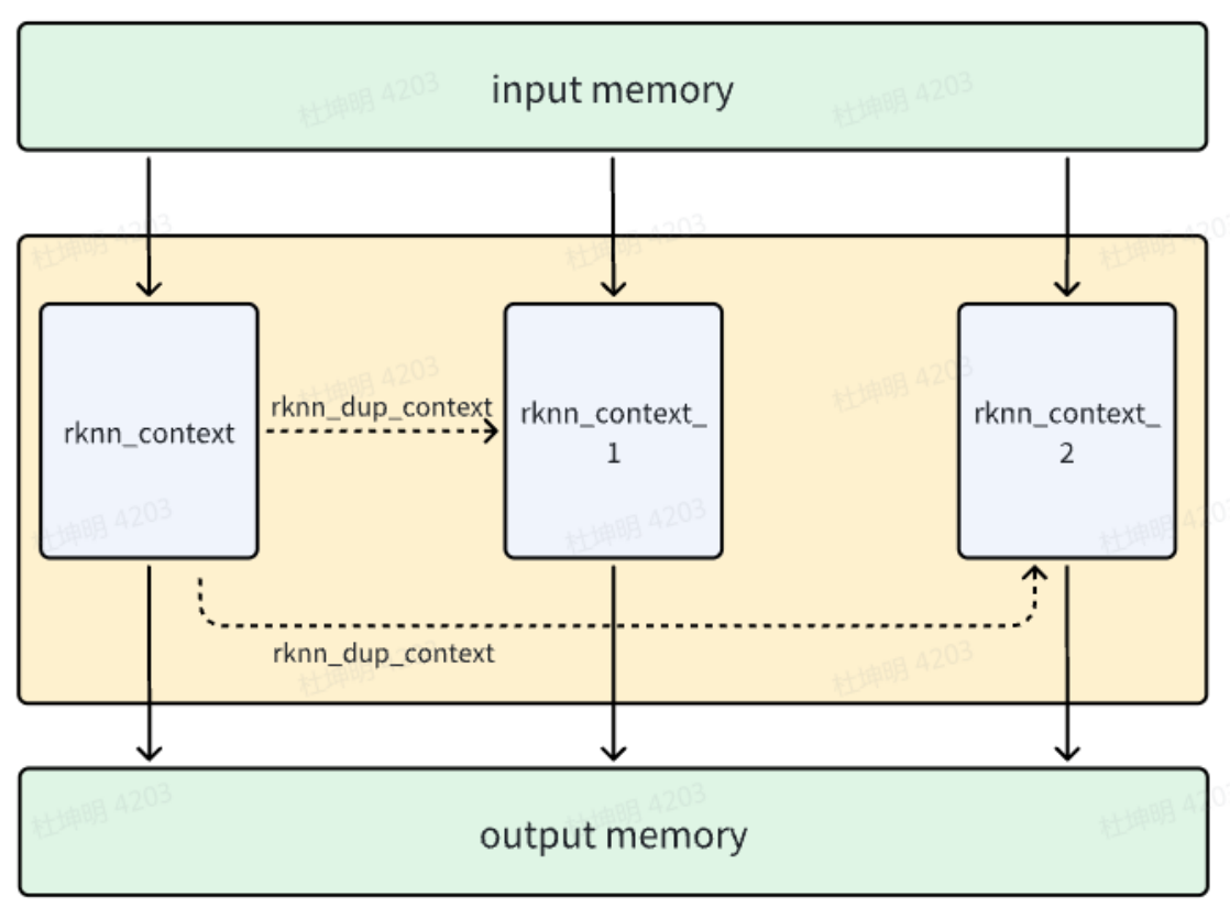
Figure 5-14 Multi-batch internal principle
5.6.2 Multi-Batch Usage
The usage of multi-batch is as follows:
1. Enable multi-batch settings on Python:
ret = rknn.build(do_quantization=True, dataset='./dataset.txt', rknn_batch_size=3)
In order to achieve optimal performance, it is recommended that rknn_batch_size be a multiple of 3 for RK3588, and a multiple of 2 for RK3576.
2. It is recommended to use zero-copy interface
5.6.3 Multi-Batch Input and Output Settings
When multi-batch function is turned on, the queried input and output size is rknn_batch_size times when it is turned off. Each context will calculate its own input offset, take input data according to this input offset for inference, then calculate its own output offset, and write its own output according to this output offset. Taking the second batch as an example, the input offset is the queried input_size divided by rknn_batch_size, and the output offset is the queried output_size divided by rknn_batch_size.
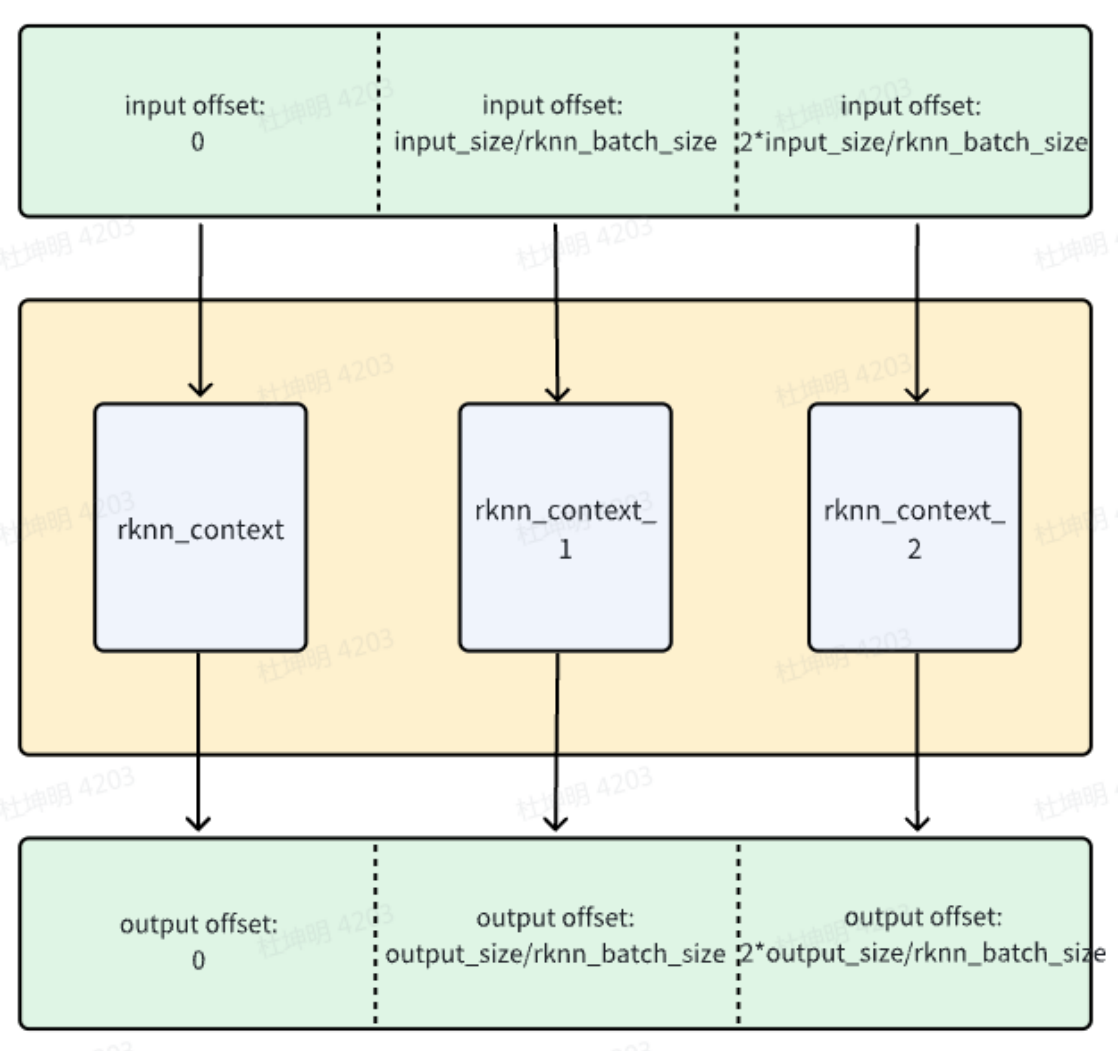
Figure 5-15 Multi-batch internal input and output address offset
5.7 RK3588/RK3576 NPU SRAM
RK3588 SOC contains 1MB of SRAM internally, of which 956KB can be used by various IPs on the SOC. It supports designated allocation for RKNPU.
RK3576 SOC contains 512KB of SRAM internally, of which 480KB can be used by various IPs on the SOC. It supports designated allocation for RKNPU.
SRAM can help RKNPU applications reduce DDR bandwidth pressure, but it may have a certain impact on inference time.
5.7.1 RKNPU Environmental Requirements
5.7.1.1 Kernel Environment Requirements
RKNPU driver version>=0.8.0
Kernel config needs to enable CONFIG_ROCKCHIP_RKNPU_SRAM=y
The Android system config path is as follows:
<path-to-your-kernel>/arch/arm64/configs/rockchip_defconfig
The Linux system config path is as follows:
<path-to-your-kernel>/arch/arm64/configs/rockchip_linux_defconfig
The corresponding DTS of the kernel needs to be allocated to RKNPU from the system SRAM.
Allocate the required size of SRAM from the system to RKNPU. The maximum size that can be allocated to RK3588 is 956KB, and the maximum size that can be allocated to RK3576 is 480KB, and the size needs to be 4K aligned.
Note: SRAM may have been allocated to other IPs in the default system, such as the codec module. The SRAM areas allocated to each IP cannot overlap, otherwise there will be data confusion caused by simultaneous reading and writing.
The following is an example of allocating 956KB to RK3588 and 480KB to RK3576 for RKNPU
RK3588:
syssram: sram@ff001000 {
  compatible = "mmio-sram";
  reg = <0x0 0xff001000 0x0 0xef000>;

  #address-cells = <1>;
  #size-cells = <1>;
  ranges = <0x0 0x0 0xff001000 0xef000>;
  /* Allocate RKNPU SRAM /
  / start address and size should be 4k algin */
  rknpu_sram: rknpu_sram@0 {
    reg = <0x0 0xef000>; // 956KB
  };
};
Mount the allocated SRAM to the RKNPU node and modify the dtsi file as shown below:
<path-to-your-kernel>/arch/arm64/boot/dts/rockchip/rk3588s.dtsi
rknpu: npu@fdab0000 {
  compatible = "rockchip,rk3588-rknpu";
  /* ... /
  / Add reference RKNPU sram */
  rockchip,sram = <&rknpu_sram>;
  status = "disabled";
};
RK3576:
sram: sram@3ff88000 {
  compatible = "mmio-sram";
  reg = <0x0 0x3ff88000 0x0 0x78000>;

  #address-cells = <1>;
  #size-cells = <1>;
  ranges = <0x0 0x0 0x3ff88000 0x78000>;
  /* Allocate RKNPU SRAM /
  / start address and size should be 4k algin */
  rknpu_sram: rknpu-sram@0 {
      reg = <0x0 0x78000>; // 480KB
  };
};
Mount the allocated SRAM to the RKNPU node and modify the dtsi file as shown below:
<path-to-your-kernel>/arch/arm64/boot/dts/rockchip/rk3576.dtsi
rknpu: npu@27700000 {
  compatible = "rockchip,rk3576-rknpu";
  /* ... /
  / Add reference RKNPU sram */
  rockchip,sram = <&rknpu_sram>;
  status = "disabled";
};
5.7.1.2 RKNN SDK Version Requirments
RKNPU Runtime library (librknnrt.so) version >=1.6.0
5.7.2 Usage
Specify RKNN_FLAG_ENABLE_SRAM in the flags parameter of the rknn_init() interface to enable SRAM in this context.
For example:
ret = rknn_init(&ctx, rknn_model, size, RKNN_FLAG_ENABLE_SRAM, NULL);
When RKNN_FLAG_ENABLE_SRAM is set, as much memory as possible will be allocated from the system’s available SRAM as the model’s Internal Tensor memory.
Note:
When SRAM is occupied by a certain rknn context, other rknn contexts do not support reusing the SRAM of this segment. The RKNN_FLAG_SHARE_SRAM function in rknn_api.h has not yet been implemented.
When a certain rknn context does not occupy all the SRAM, the remaining SRAM can be used by other rknn contexts.
5.7.3 Debug
5.7.3.1 Query SRAM Enable
Check whether SRAM is enabled through the boot kernel log, including the address range and size information of the SRAM specified for RKNPU, as shown below:
rk3588_s:/ # dmesg | grep rknpu -i
RKNPU fdab0000.npu: RKNPU: sram region: [0x00000000ff001000, 0x00000000ff0f0000), sram size: 0xef000
5.7.3.2 Query SRAM Usage
SRAM usage can be queried through nodes
The following is a bit chart of unused SRAM, each point represents 4K size
rk3588_s:/ # cat /sys/kernel/debug/rknpu/mm
SRAM bitmap: "*" - used, "." - free (1bit = 4KB)
[000] [................................]
[001] [................................]
[002] [................................]
[003] [................................]
[004] [................................]
[005] [................................]
[006] [................................]
[007] [...............]
SRAM total size: 978944, used: 0, free: 978944
# Unit is Byte
The following is a bit chart after using 512KB SRAM
rk3588_s:/ # cat /sys/kernel/debug/rknpu/mm
SRAM bitmap: "*" - used, "." - free (1bit = 4KB)
[000] [********************************]
[001] [********************************]
[002] [********************************]
[003] [********************************]
[004] [................................]
[005] [................................]
[006] [................................]
[007] [...............]
SRAM total size: 978944, used: 524288, free: 454656
# Unit is Byte
5.7.3.3 Query SRAM Size Through RKNN API
Query SRAM size information through the RKNN_QUERY_MEM_SIZE interface of rknn_query()
typedef struct _rknn_mem_size {
  uint32_t total_weight_size;
  uint32_t total_internal_size;
  uint64_t total_dma_allocated_size;
  uint32_t total_sram_size;
  uint32_t free_sram_size;
  uint32_t reserved[10];
} rknn_mem_size;
Among total_sram_size indicates the total size of SRAM allocated by the system to RKNPU, unit is Byte.
free_sram_size indicates the size of SRAM that can be used by the remaining RKNPU, unit is Byte
5.7.3.4 Query Model SRAM Occupancy
In the RKNPU device environment, set the following environment variables before running the RKNN application to print the SRAM usage prediction:
export RKNN_LOG_LEVEL=3
Layer occupancy of Internal allocated SRAM, as shown in the following log:
---------------------------------------------------------------------------
Total allocated Internal SRAM Size: 524288, Addr: [0xff3e0000, 0xff460000)
---------------------------------------------------------------------------
---------------------------------------------------------------------+----------------------------------+-----------
ID User Tensor DataType OrigShape NativeShape | [Start End) Size | SramHit
---------------------------------------------------------------------+----------------------------------+-----------
1 ConvRelu input0 INT8 (1,3,224,224) (1,1,224,224,3) | 0xff3b0000 0xff3d4c00 0x00024c00 | \
2 ConvRelu output2 INT8 (1,32,112,112) (1,2,112,112,16) | 0xff404c00 0xff466c00 0x00062000 |
0x0005b400
3 ConvRelu output4 INT8 (1,32,112,112) (1,4,112,112,16) | 0xff466c00 0xff52ac00 0x000c4000 |
0x00000000
4 ConvRelu output6 INT8 (1,64,112,112) (1,4,112,112,16) | 0xff52ac00*0xff5eec00 0x000c4000 |
0x00000000
5 ConvRelu output8 INT8 (1,64,56,56) (1,4,56,56,16) | 0xff3e0000 0xff411000 0x00031000 |
0x00031000
6 ConvRelu output10 INT8 (1,128,56,56) (1,8,56,56,16) | 0xff411000 0xff473000 0x00062000 |
0x0004f000
7 ConvRelu output12 INT8 (1,128,56,56) (1,8,56,56,16) | 0xff473000 0xff4d5000 0x00062000 |
0x00000000
8 ConvRelu output14 INT8 (1,128,56,56) (1,8,56,56,16) | 0xff3e0000 0xff442000 0x00062000 |
0x00062000
9 ConvRelu output16 INT8 (1,128,28,28) (1,8,28,28,16) | 0xff442000 0xff45a800 0x00018800 |
0x00018800
10 ConvRelu output18 INT8 (1,256,28,28) (1,16,28,28,16) | 0xff3e0000 0xff411000 0x00031000 |
0x00031000
11 ConvRelu output20 INT8 (1,256,28,28) (1,16,28,28,16) | 0xff411000 0xff442000 0x00031000 |
0x00031000
12 ConvRelu output22 INT8 (1,256,28,28) (1,16,28,28,16) | 0xff3e0000 0xff411000 0x00031000 |
0x00031000
13 ConvRelu output24 INT8 (1,256,14,14) (1,16,14,14,16) | 0xff411000 0xff41d400 0x0000c400 |
0x0000c400
14 ConvRelu output26 INT8 (1,512,14,14) (1,32,14,14,16) | 0xff3e0000 0xff3f8800 0x00018800 |
0x00018800
15 ConvRelu output28 INT8 (1,512,14,14) (1,32,14,14,16) | 0xff3f8800 0xff411000 0x00018800 |
0x00018800
16 ConvRelu output30 INT8 (1,512,14,14) (1,32,14,14,16) | 0xff3e0000 0xff3f8800 0x00018800 |
0x00018800
17 ConvRelu output32 INT8 (1,512,14,14) (1,32,14,14,16) | 0xff3f8800 0xff411000 0x00018800 |
0x00018800
18 ConvRelu output34 INT8 (1,512,14,14) (1,32,14,14,16) | 0xff3e0000 0xff3f8800 0x00018800 |
0x00018800
19 ConvRelu output36 INT8 (1,512,14,14) (1,32,14,14,16) | 0xff3f8800 0xff411000 0x00018800 |
0x00018800
20 ConvRelu output38 INT8 (1,512,14,14) (1,32,14,14,16) | 0xff3e0000 0xff3f8800 0x00018800 |
0x00018800
21 ConvRelu output40 INT8 (1,512,14,14) (1,32,14,14,16) | 0xff3f8800 0xff411000 0x00018800 |
0x00018800
22 ConvRelu output42 INT8 (1,512,14,14) (1,32,14,14,16) | 0xff3e0000 0xff3f8800 0x00018800 |
0x00018800
23 ConvRelu output44 INT8 (1,512,14,14) (1,32,14,14,16) | 0xff3f8800 0xff411000 0x00018800 |
0x00018800
24 ConvRelu output46 INT8 (1,512,14,14) (1,32,14,14,16) | 0xff3e0000 0xff3f8800 0x00018800 |
0x00018800
25 ConvRelu output48 INT8 (1,512,7,7) (1,33,7,7,16) | 0xff3f8800 0xff3ff000 0x00006800 | 0x00006800
26 ConvRelu output50 INT8 (1,1024,7,7) (1,67,7,7,16) | 0xff3e0000 0xff3ed000 0x0000d000 |
0x0000d000
27 ConvRelu output52 INT8 (1,1024,7,7) (1,67,7,7,16) | 0xff3ed000 0xff3fa000 0x0000d000 |
0x0000d000
28 AveragePool output54 INT8 (1,1024,7,7) (1,67,7,7,16) | 0xff3e0000 0xff3ed000 0x0000d000 |
0x0000d000
29 Conv output55 INT8 (1,1024,1,1) (1,64,1,1,16) | 0xff3ed000 0xff3ed400 0x00000400 | 0x00000400
30 Softmax output56 INT8 (1,1000,1,1) (1,64,1,1,16) | 0xff3e0000 0xff3e0400 0x00000400 |
0x00000400
31 OutputOperator output57 FLOAT (1,1000,1,1) (1,1000,1,1) | 0xff3ae000 0xff3aefa0 0x00000fa0 | \
---------------------------------------------------------------------+----------------------------------+-----------
----------------------------------------
Total Weight Memory Size: 4260864
Total Internal Memory Size: 2157568
Predict Internal Memory RW Amount: 11068320
Predict Weight Memory RW Amount: 4260832
Predict SRAM Hit RW Amount: 6688768
----------------------------------------
The SRAM Hit in the text chart above is the SRAM size occupied by the current layer tensor, which means that compared with not turning on SRAM, the amount of DDR read and write data corresponding to size will be saved.
Predict SRAM Hit RW Amount is the read and write prediction of the entire model SRAM, indicating the amount of DDR read and write data that can be saved in each frame compared with SRAM not turned on.
Note: Linux environment logs are redirected to the terminal, and Android environment logs are redirected to logcat.
5.8 Model Pruning
Model pruning can generally be divided into two methods: lossy pruning and lossless pruning. The model pruning of RKNN-Toolkit2 is lossless pruning, which means that it can reduce the size of the model and the amount of calculation without degrading floating point accuracy of the model. And the quantization accuracy of the model can even be improved.
However, not all models can be used for lossless pruning. Lossless pruning is based on the degree of sparseness of the model’s weights to remove some weights and feature channels that have no impact on the model, results to reduce the size and the calculation of the model After the model pruning configuration is enabled (set the model_pruning parameter of rknn.config() to True), the model will be automatically pruned according to the degree of weight sparsification during model conversion.
If the model is pruned successfully, the results will be printed, as follows:
I model_pruning results:

I Weight: -1.12145 MB (-6.9%)

I GFLOPs: -0.15563 (-13.4%)
Among Weight cut off 1.12145 MB (accounting for 6.9%), and the model calculation was reduced by 0.15563 GFLOPs (accounting for 13.4%).
If pruning fails due to insufficient model sparsity, no processing will be done (nor will the above information be printed), so this configuration will not affect normal model conversion.
5.9 Model Encryption
Model encryption refers to further processing it after generating the RKNN model. Using the model generated by rknn.export_rknn(), the graph structure can be viewed through third-party tools such as Netron. After the model is encrypted, third-party tools such as Netron will not be able to view the corresponding network structure and obtain weights, which will protect the model. The current encrypted RKNN model can be used in the same way as the unencrypted model. There is no need to make any modifications during RKNPU device inference. Password protection will be considered in the future.
Usage as follows:
# Create RKNN object
rknn = RKNN()
# Export encrypted RKNN model
crypt_level= 1
ret = rknn.export_encrypted_rknn_model("input.rknn", "encrypt.rknn", crypt_level)
if ret != 0:
  print('Encrypt RKNN model failed!')
crypt_level is used to specify the encryption level, which has three levels: 1, 2 and 3. The default value is 1. The higher the level, the higher the security and the more time-consuming decryption, vice versa.
Supported platforms: RK3562/RK3566/RK3568/RK3576/RK3588/RV1126B
5.10 Cacheable memory consistency
The Cacheable memory consistency problem means that when both the CPU and NPU devices access the same memory with cache flag, the CPU will cache the data into the data cache. If the DDR data accessed by the NPU is inconsistent with the CPU cache, it will cause data reading errors. Therefore, it is necessary to call the refresh cache interface to ensure that the DDR memory data accessed by the CPU and NPU is consistent. This chapter introduces the direction of synchronized data and how to use the rknn_mem_sync interface to refresh the cache.
5.10.1 Direction of cacheable memory synchronization
When the CPU writes data to the cacheable memory, and then when the NPU accesses the memory, it must ensure that the data in the CPU cache is synchronized to the DDR. The direction of synchronization at this time is from the CPU to the NPU device; when the NPU finishes writing the data, the CPU begins to access the memory. When accessing memory, ensure that the DDR data is consistent with the data in the CPU cache. At this time, the direction of synchronization is from the NPU device to the CPU. RKNN C API provides the rknn_mem_sync_mode enumeration type to indicate the direction of cacheable memory synchronization. The data structure is as follows:
/*
  The mode to sync cacheable rknn memory.
*/
typedef enum _rknn_mem_sync_mode {
RKNN_MEMORY_SYNC_TO_DEVICE = 0x1, /* the mode used for consistency of device access after CPU accesses
data. */
RKNN_MEMORY_SYNC_FROM_DEVICE = 0x2, /* the mode used for consistency of CPU access after device
accesses data. */
RKNN_MEMORY_SYNC_BIDIRECTIONAL =
  RKNN_MEMORY_SYNC_TO_DEVICE | RKNN_MEMORY_SYNC_FROM_DEVICE, /* the mode used for
consistency of data access
between device and CPU in both directions. */
} rknn_mem_sync_mode;
RKNN_MEMORY_SYNC_TO_DEVICE: Indicates that the data synchronization direction is from CPU to NPU device
RKNN_MEMORY_SYNC_FROM_DEVICE: Indicates that the data synchronization direction is from NPU device to CPU
RKNN_MEMORY_SYNC_BIDIRECTIONAL: Indicates that data is synchronized in both directions between NPU and CPU. This enumeration can be used when the user is not sure about the direction of synchronized data.
When clarifying the data synchronization direction, it is recommended to use the one-way CPU cache refresh mode to avoid performance losses caused by redundant CPU cache refresh actions.
5.10.2 Synchronizing cacheable memory
After clarifying the data synchronization direction, you can use the rknn_mem_sync interface to synchronize the cacheable memory. The interface form is as follows:
int rknn_mem_sync(rknn_context context, rknn_tensor_mem* mem, rknn_mem_sync_mode mode);
Among them, context is the context (set to NULL by default on non-RV1103/RV1103B/RV1106/RV1106B platforms), mem is the rknn_tensor_mem* pointer type returned by the rknn_create_mem interface, and mode refers to the direction of synchronized data.
5.11 Model Sparse Inference
This function is used by the Torch model to automatically sparse the model weights during the training phase and use RKNN for sparse reasoning, thereby reduce model inference time. Currently the function only supports RK3576.
5.11.1 Sparsity Principle
The model weight sparseness is reset to zero in a user-defined manner during the training. The specific methods include 4:2 input direction sparsification, 4:2 output direction sparsification, 16:4 input and output sparsification, and 16:4 sparsification. Output and input sparsification. The implementation principle of 4:2 input direction sparsification is shown in Figure 5-16. Set the model weight along the input direction and select two of the four consecutive values to zero. It should be noted that when the specified direction of the training sparse model weight is not 4-aligned, a padding operation will be performed and the number of sparse weight channels must be greater than 32 to take effect.
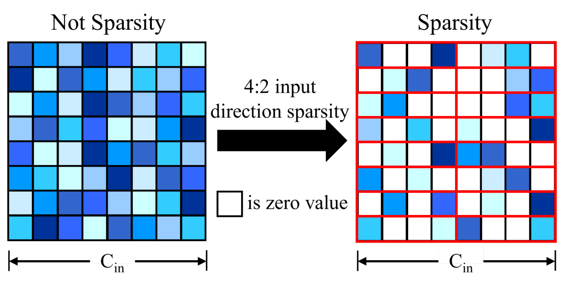
Figure 5-16 4:2 input direction sparsity principle diagram
The four types of weight sparse descriptions are shown in Table 5-10, where the input and output directions are the directions of the weights. For example, the 2-dimensional convolution shape is C_out × C_in × K_h × K_w, the input direction is C_in, and the output direction is C_out. In the method with a sparsity rate of 75%, the pre-training model can be an unsparse model or a sparse model. It is recommended to use a 4:2 input/output direction sparsification model as the pre-training model to reduce the accuracy loss after sparsification.
Table 5-10 Model weight sparsification instructions
| Sparsification method | Sparsity rate |
Specification |
|---|---|---|
| 4:2 input direction sparsification |
50% | Sparse the weights along the input direction |
| 4:2 output direction sparsification |
50% | Sparse the weights along the output direction |
| 16:4 input and output sparsification |
75% | First sparse 4:2 along the input direction, then sparse 4:2 along the output direction |
| 16:4 output and input sparsification |
75% | First sparse 4:2 along the output direction, then sparse 4:2 along the input direction |
5.11.2 Training the sparse model
1. First make sure that cuda can be used and install the autosparsity package
pip install autosparsity-1.0-cp38-cp38m-linux_x86_64.whl
The autosparsity installation package path is https://github.com/airockchip/rknn-toolkit2/tree/master/autospa rsity/packages
2. Take the 4:2 input direction sparsification of resnet50 in torchvision as an example to autosparsity
import torch
import torchvision.models as models
from autosparsity.sparsity import sparsity_model

if __name__ == "__main__":
  model = models.resnet50(pretrained=True).cuda()
  optimizer = None
  mode = 0
  sparsity_model(model, optimizer, mode)
  model.eval()
  x = torch.randn((1,3,224,224)).cuda()
  torch.onnx.export(
  model, x, 'resnet50.onnx', input_names=['inputs'], output_names=['outputs']
  )
To sparsify a custom model, just add the sparsity_model function before model training. The reference example is as follows:
# insert model autosparsity code before training
import torch
import torchvision.models as models
from autosparsity.sparsity import sparsity_model

...

model = models.resnet34(pretrained=True).cuda()
mode = 0
sparsity_model(model, optimizer, mode)

# normal training
x, y = DataLoader(args)
for epoch in range(epochs):
  y_pred = model(x)
  loss = loss_func(y_pred, y)
  loss.backward()
  optimizer.step()
  ...
Note: Attention model sparse training relies on a trained front-end model. Therefore, before doing sparse training, please first train a model with “good” effect, and perform sparse training based on this model.
The parameter description of the sparsity_model function is as follows:
Table 5-11 Description of parameters of sparsity_model function
| Parameters | Specification |
|---|---|
| model | Original training model |
| optimizer | Original optimizer, default None |
| mode | Sparsification method, optional values are 0, 1, 2, 3, default is 0 0: 4:2 input direction sparsification(50% sparsity rate) 1: 4:2 output direction sparsification(50% sparsity rate) 2: 16:4 input and output sparsification(75% sparsity rate) 3: 16:4 output and input sparsification(75% sparsity rate) |
| verbose | Log level, optional values are 0, 1, 2, default is 2 0: Errors 1: Errors and Warnings 2: Errors, warnings and info |
| whitelist | List of modules supported by sparsification, supporting 1d conv, 2d conv, 3d conv, linear, MultiheadAttention, default [torch.nn.Linear, torch.nn.Conv2d] |
| allowed_layer_names | The layer name that allows sparsification. When the user configures it, only the allowed layers will be sparse. The default is None. |
| disallowed_layer_names | Sparse layer names are not allowed. This layer will be skipped when configured by the user. Default [] |
| fast | Set to True to use a fast method to calculate the mask, the default is False (the default mask calculation method will be invalid for some models, if sparse error is reported, try setting this parameter to True) |
5.11.3 RKNN Sparse Inference Usage
Set the opening and closing of model sparseness through the “sparse_infer” parameter of the config() interface in RKNN-Toolkit2. The corresponding parameter is True/False, and the default is False. The reference code to enable sparse inference is as follows:
rknn.config(target_platform=’rk3576’, sparse_infer=True)
The complete sparse inference of Python code can be found at: https://github.com/airockchip/rknn-toolkit2/tree/m aster/autosparsity/examples
When deploying using the C API, first use RKNN-Toolkit2 to set the “sparse_infer” parameter to True in the config() interface to generate an RKNN model with sparse inferencing, and then call the general API interface process or zero-copy interface process normally.
When using Python code for inference, you can set verbose=True when building the RKNN object to enable log printing of the sparseness of each layer. When using the C API for inference, set the environment variable RKNN_LOG_LEVEL=4 to enable log printing of the sparseness of each layer. The log information is as follows:
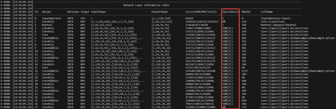
| Log prefix | ID | OpType | DataType | Target | InputShape | OutputShape | Cycles(DDR/NPU/Total) | SparseRatio | RW(KB) | FullName |
|---|---|---|---|---|---|---|---|---|---|---|
| D RKNN: [14:58:09.324] | 0 | InputOperator | INT8 | CPU | \ | (1,3,224,224) | 0/0/0 | \ | 0 | InputOperator:inputs |
| D RKNN: [14:58:09.324] | 1 | ConvRelu | INT8 | NPU | (1,3,224,224),(64,3,7,7),(64) | (1,64,112,112) | 129458/1229312/1229312 | 0% | 159 | Conv:/conv1/Conv |
| D RKNN: [14:58:09.324] | 2 | MaxPool | INT8 | NPU | (1,64,112,112) | (1,64,56,56) | 134430/0/134430 | \ | 784 | MaxPool:/maxpool/MaxPool |
| D RKNN: [14:58:09.324] | 3 | ConvRelu | INT8 | NPU | (1,64,56,56),(64,32,1,1),(64) | (1,64,56,56) | 53807/25088/53807 | 50%(IC) | 196 | Conv:/layer1/layer1.0/conv1/Conv |
| D RKNN: [14:58:09.324] | 4 | ConvRelu | INT8 | NPU | (1,64,56,56),(64,32,3,3),(64) | (1,64,56,56) | 53532/112896/112896 | 50%(IC) | 194 | Conv:/layer1/layer1.0/conv2/Conv |
| D RKNN: [14:58:09.324] | 5 | Conv | INT8 | NPU | (1,64,56,56),(256,32,1,1),(256) | (1,256,56,56) | 134568/100352/134568 | 50%(IC) | 197 | Conv:/layer1/layer1.0/conv3/Conv |
| D RKNN: [14:58:09.324] | 6 | ConvAddRelu | INT8 | NPU | (1,64,56,56),(256,32,1,1),(256),… | (1,256,56,56) | 242112/100352/242112 | 50%(IC) | 981 | Conv:/layer1/layer1.0/downsample/downsample.0/Conv |
| D RKNN: [14:58:09.324] | 7 | ConvRelu | INT8 | NPU | (1,256,56,56),(64,128,1,1),(64) | (1,64,56,56) | 134362/50176/134362 | 50%(IC) | 783 | Conv:/layer1/layer1.1/conv1/Conv |
| D RKNN: [14:58:09.324] | 8 | ConvRelu | INT8 | NPU | (1,64,56,56),(64,32,3,3),(64) | (1,64,56,56) | 53532/112896/112896 | 50%(IC) | 194 | Conv:/layer1/layer1.1/conv2/Conv |
| D RKNN: [14:58:09.324] | 9 | ConvAddRelu | INT8 | NPU | (1,64,56,56),(256,32,1,1),(256),… | (1,256,56,56) | 242112/100352/242112 | 50%(IC) | 981 | Conv:/layer1/layer1.1/conv3/Conv |
| D RKNN: [14:58:09.324] | 10 | ConvRelu | INT8 | NPU | (1,256,56,56),(64,128,1,1),(64) | (1,64,56,56) | 134362/50176/134362 | 50%(IC) | 783 | Conv:/layer1/layer1.2/conv1/Conv |
| D RKNN: [14:58:09.324] | 11 | ConvRelu | INT8 | NPU | (1,64,56,56),(64,32,3,3),(64) | (1,64,56,56) | 53532/112896/112896 | 50%(IC) | 194 | Conv:/layer1/layer1.2/conv2/Conv |
| D RKNN: [14:58:09.324] | 12 | ConvAddRelu | INT8 | NPU | (1,64,56,56),(256,32,1,1),(256),… | (1,256,56,56) | 242112/100352/242112 | 50%(IC) | 981 | Conv:/layer1/layer1.2/conv3/Conv |
| D RKNN: [14:58:09.324] | 13 | ConvRelu | INT8 | NPU | (1,256,56,56),(128,128,1,1),(128) | (1,128,56,56) | 161179/100352/161179 | 50%(IC) | 783 | Conv:/layer2/layer2.0/conv1/Conv |
| D RKNN: [14:58:09.324] | 14 | ConvRelu | INT8 | NPU | (1,128,56,56),(128,64,3,3),(128) | (1,128,28,28) | 66118/112896/112896 | 50%(IC) | 384 | Conv:/layer2/layer2.0/conv2/Conv |
| D RKNN: [14:58:09.324] | 15 | Conv | INT8 | NPU | (1,128,28,28),(512,64,1,1),(512) | (1,512,28,28) | 67215/50176/67215 | 50%(IC) | 98 | Conv:/layer2/layer2.0/conv3/Conv |
| D RKNN: [14:58:09.324] | 16 | ConvAddRelu | INT8 | NPU | (1,256,56,56),(512,128,1,1),(512),… | (1,512,28,28) | 214540/100352/214540 | 50%(IC) | 1172 | Conv:/layer2/layer2.0/downsample/downsample.0/Conv |
| D RKNN: [14:58:09.324] | 17 | ConvRelu | INT8 | NPU | (1,512,28,28),(128,256,1,1),(128) | (1,128,28,28) | 66804/50176/66804 | 50%(IC) | 389 | Conv:/layer2/layer2.1/conv1/Conv |
| D RKNN: [14:58:09.324] | 18 | ConvRelu | INT8 | NPU | (1,128,28,28),(128,64,3,3),(128) | (1,128,28,28) | 25789/112896/112896 | 50%(IC) | 90 | Conv:/layer2/layer2.1/conv2/Conv |
| D RKNN: [14:58:09.324] | 19 | ConvAddRelu | INT8 | NPU | (1,128,28,28),(512,64,1,1),(512),… | (1,512,28,28) | 120988/50176/120988 | 50%(IC) | 490 | Conv:/layer2/layer2.1/conv3/Conv |
| D RKNN: [14:58:09.324] | 20 | ConvRelu | INT8 | NPU | (1,512,28,28),(128,256,1,1),(128) | (1,128,28,28) | 66804/50176/66804 | 50%(IC) | 389 | Conv:/layer2/layer2.2/conv1/Conv |
| D RKNN: [14:58:09.324] | 21 | ConvRelu | INT8 | NPU | (1,128,28,28),(128,64,3,3),(128) | (1,128,28,28) | 25789/112896/112896 | 50%(IC) | 90 | Conv:/layer2/layer2.2/conv2/Conv |
| D RKNN: [14:58:09.324] | 22 | ConvAddRelu | INT8 | NPU | (1,128,28,28),(512,64,1,1),(512),… | (1,512,28,28) | 120988/50176/120988 | 50%(IC) | 490 | Conv:/layer2/layer2.2/conv3/Conv |
| D RKNN: [14:58:09.324] | 23 | ConvRelu | INT8 | NPU | (1,512,28,28),(128,256,1,1),(128) | (1,128,28,28) | 66804/50176/66804 | 50%(IC) | 389 | Conv:/layer2/layer2.3/conv1/Conv |
| D RKNN: [14:58:09.324] | 24 | ConvRelu | INT8 | NPU | (1,128,28,28),(128,64,3,3),(128) | (1,128,28,28) | 25789/112896/112896 | 50%(IC) | 90 | Conv:/layer2/layer2.3/conv2/Conv |
| D RKNN: [14:58:09.324] | 25 | ConvAddRelu | INT8 | NPU | (1,128,28,28),(512,64,1,1),(512),… | (1,512,28,28) | 120988/50176/120988 | 50%(IC) | 490 | Conv:/layer2/layer2.3/conv3/Conv |
| D RKNN: [14:58:09.324] | 26 | ConvRelu | INT8 | NPU | (1,512,28,28),(256,256,1,1),(256) | (1,256,28,28) | 79835/100352/100352 | 50%(IC) | 386 | Conv:/layer3/layer3.0/conv1/Conv |
| D RKNN: [14:58:09.324] | 27 | ConvRelu | INT8 | NPU | (1,256,28,28),(256,256,3,3),(256) | (1,256,14,14) | 112894/119808/119808 | 0% | 774 | Conv:/layer3/layer3.0/conv2/Conv |
Figure 5-17 4:2 input direction sparse Python printing log
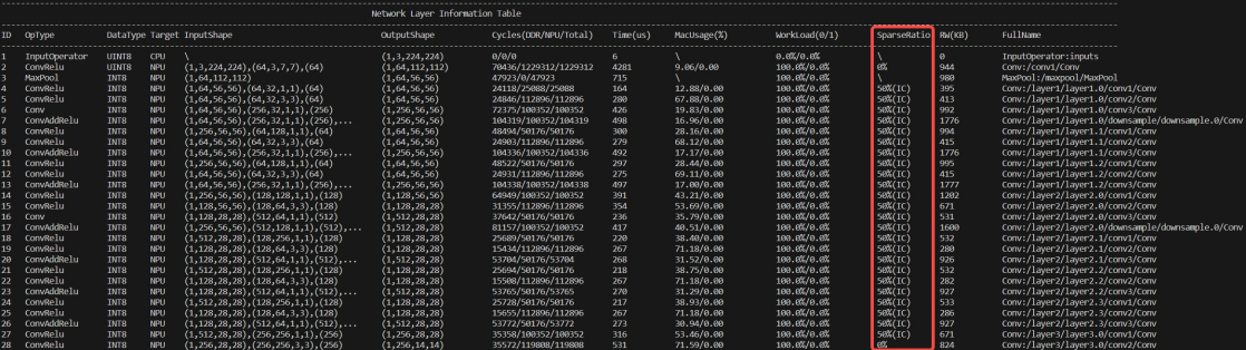
| ID | OpType | DataType | Target | InputShape | OutputShape | Cycles(DDR/NPU/Total) | Time(us) | MacUsage(%) | WorkLoad(0/1) | SparseRatio | RW(KB) | FullName |
|---|---|---|---|---|---|---|---|---|---|---|---|---|
| 1 | InputOperator | UINT8 | CPU | \ | (1,3,224,224) | 0/0/0 | 6 | \ | 0.0%/0.0% | \ | 0 | InputOperator:inputs |
| 2 | ConvRelu | INT8 | NPU | (1,3,224,224),(64,3,7,7),(64) | (1,64,112,112) | 70436/1229312/1229312 | 4281 | 9.06/0.00 | 100.0%/0.0% | 0% | 944 | Conv:/conv1/Conv |
| 3 | MaxPool | INT8 | NPU | (1,64,112,112) | (1,64,56,56) | 47923/0/47923 | 715 | \ | 100.0%/0.0% | \ | 980 | MaxPool:/maxpool/MaxPool |
| 4 | ConvRelu | INT8 | NPU | (1,64,56,56),(64,32,1,1),(64) | (1,64,56,56) | 24118/25088/25088 | 164 | 12.88/0.00 | 100.0%/0.0% | 50%(IC) | 395 | Conv:/layer1/layer1.0/conv1/Conv |
| 5 | ConvRelu | INT8 | NPU | (1,64,56,56),(64,32,3,3),(64) | (1,64,56,56) | 24846/112896/112896 | 280 | 67.88/0.00 | 100.0%/0.0% | 50%(IC) | 413 | Conv:/layer1/layer1.0/conv2/Conv |
| 6 | Conv | INT8 | NPU | (1,64,56,56),(256,32,1,1),(256) | (1,256,56,56) | 72375/100352/100352 | 426 | 19.83/0.00 | 100.0%/0.0% | 50%(IC) | 992 | Conv:/layer1/layer1.0/conv3/Conv |
| 7 | ConvAddRelu | INT8 | NPU | (1,64,56,56),(256,32,1,1),(256),… | (1,256,56,56) | 104319/100352/104319 | 498 | 16.96/0.00 | 100.0%/0.0% | 50%(IC) | 1776 | Conv:/layer1/layer1.0/downsample/downsample.0/Conv |
| 8 | ConvRelu | INT8 | NPU | (1,256,56,56),(64,128,1,1),(64) | (1,64,56,56) | 48494/50176/50176 | 300 | 28.16/0.00 | 100.0%/0.0% | 50%(IC) | 994 | Conv:/layer1/layer1.1/conv1/Conv |
| 9 | ConvRelu | INT8 | NPU | (1,64,56,56),(64,32,3,3),(64) | (1,64,56,56) | 24903/112896/112896 | 279 | 68.12/0.00 | 100.0%/0.0% | 50%(IC) | 415 | Conv:/layer1/layer1.1/conv2/Conv |
| 10 | ConvAddRelu | INT8 | NPU | (1,64,56,56),(256,32,1,1),(256),… | (1,256,56,56) | 104336/100352/104336 | 492 | 17.17/0.00 | 100.0%/0.0% | 50%(IC) | 1776 | Conv:/layer1/layer1.1/conv3/Conv |
| 11 | ConvRelu | INT8 | NPU | (1,256,56,56),(64,128,1,1),(64) | (1,64,56,56) | 48522/50176/50176 | 297 | 28.44/0.00 | 100.0%/0.0% | 50%(IC) | 995 | Conv:/layer1/layer1.2/conv1/Conv |
| 12 | ConvRelu | INT8 | NPU | (1,64,56,56),(64,32,3,3),(64) | (1,64,56,56) | 24931/112896/112896 | 275 | 69.11/0.00 | 100.0%/0.0% | 50%(IC) | 415 | Conv:/layer1/layer1.2/conv2/Conv |
| 13 | ConvAddRelu | INT8 | NPU | (1,64,56,56),(256,32,1,1),(256),… | (1,256,56,56) | 104338/100352/104338 | 497 | 17.00/0.00 | 100.0%/0.0% | 50%(IC) | 1777 | Conv:/layer1/layer1.2/conv3/Conv |
| 14 | ConvRelu | INT8 | NPU | (1,256,56,56),(128,128,1,1),(128) | (1,128,56,56) | 64949/100352/100352 | 391 | 43.21/0.00 | 100.0%/0.0% | 50%(IC) | 1202 | Conv:/layer2/layer2.0/conv1/Conv |
| 15 | ConvRelu | INT8 | NPU | (1,128,56,56),(128,64,3,3),(128) | (1,128,28,28) | 31355/112896/112896 | 354 | 53.69/0.00 | 100.0%/0.0% | 50%(IC) | 671 | Conv:/layer2/layer2.0/conv2/Conv |
| 16 | Conv | INT8 | NPU | (1,128,28,28),(512,64,1,1),(512) | (1,512,28,28) | 37642/50176/50176 | 236 | 35.79/0.00 | 100.0%/0.0% | 50%(IC) | 531 | Conv:/layer2/layer2.0/conv3/Conv |
| 17 | ConvAddRelu | INT8 | NPU | (1,256,56,56),(512,128,1,1),(512),… | (1,512,28,28) | 81157/100352/100352 | 417 | 40.51/0.00 | 100.0%/0.0% | 50%(IC) | 1600 | Conv:/layer2/layer2.0/downsample/downsample.0/Conv |
| 18 | ConvRelu | INT8 | NPU | (1,512,28,28),(128,256,1,1),(128) | (1,128,28,28) | 25689/50176/50176 | 220 | 38.40/0.00 | 100.0%/0.0% | 50%(IC) | 532 | Conv:/layer2/layer2.1/conv1/Conv |
| 19 | ConvRelu | INT8 | NPU | (1,128,28,28),(128,64,3,3),(128) | (1,128,28,28) | 15434/112896/112896 | 267 | 71.18/0.00 | 100.0%/0.0% | 50%(IC) | 280 | Conv:/layer2/layer2.1/conv2/Conv |
| 20 | ConvAddRelu | INT8 | NPU | (1,128,28,28),(512,64,1,1),(512),… | (1,512,28,28) | 53704/50176/53704 | 268 | 31.52/0.00 | 100.0%/0.0% | 50%(IC) | 926 | Conv:/layer2/layer2.1/conv3/Conv |
| 21 | ConvRelu | INT8 | NPU | (1,512,28,28),(128,256,1,1),(128) | (1,128,28,28) | 25694/50176/50176 | 218 | 38.75/0.00 | 100.0%/0.0% | 50%(IC) | 532 | Conv:/layer2/layer2.2/conv1/Conv |
| 22 | ConvRelu | INT8 | NPU | (1,128,28,28),(128,64,3,3),(128) | (1,128,28,28) | 15508/112896/112896 | 267 | 71.18/0.00 | 100.0%/0.0% | 50%(IC) | 282 | Conv:/layer2/layer2.2/conv2/Conv |
| 23 | ConvAddRelu | INT8 | NPU | (1,128,28,28),(512,64,1,1),(512),… | (1,512,28,28) | 53765/50176/53765 | 270 | 31.29/0.00 | 100.0%/0.0% | 50%(IC) | 927 | Conv:/layer2/layer2.2/conv3/Conv |
| 24 | ConvRelu | INT8 | NPU | (1,512,28,28),(128,256,1,1),(128) | (1,128,28,28) | 25728/50176/50176 | 217 | 38.93/0.00 | 100.0%/0.0% | 50%(IC) | 533 | Conv:/layer2/layer2.3/conv1/Conv |
| 25 | ConvRelu | INT8 | NPU | (1,128,28,28),(128,64,3,3),(128) | (1,128,28,28) | 15655/112896/112896 | 267 | 71.18/0.00 | 100.0%/0.0% | 50%(IC) | 286 | Conv:/layer2/layer2.3/conv2/Conv |
| 26 | ConvAddRelu | INT8 | NPU | (1,128,28,28),(512,64,1,1),(512),… | (1,512,28,28) | 53772/50176/53772 | 273 | 30.94/0.00 | 100.0%/0.0% | 50%(IC) | 927 | Conv:/layer2/layer2.3/conv3/Conv |
| 27 | ConvRelu | INT8 | NPU | (1,512,28,28),(256,256,1,1),(256) | (1,256,28,28) | 35358/100352/100352 | 316 | 53.46/0.00 | 100.0%/0.0% | 50%(IC) | 671 | Conv:/layer3/layer3.0/conv1/Conv |
| 28 | ConvRelu | INT8 | NPU | (1,256,28,28),(256,256,3,3),(256) | (1,256,14,14) | 35572/119808/119808 | 531 | 71.59/0.00 | 100.0%/0.0% | 0% | 824 | Conv:/layer3/layer3.0/conv2/Conv |
Figure 5-18 4:2 input direction sparse C API printing log
Among them, SparseRation represents the sparse rate, 4:2 input direction sparseness corresponds to 50%(IC), 4:2 output direction sparseness corresponds to 50%(OC), 16:4 input output sparseness corresponds to 16:4 output input sparseness. 75%. 0% means no sparsification is done.
5.11.4 RKNN sparse inference restrictions
Sparse inferencing is implemented based on the NPU hardware architecture. Limited by hardware specifications, the sparse inference of RK3576 currently only supports 2d Conv and the group parameter is 1. The other restrictions are as follows:
Table 5-12 RK3576 sparse inference restrictions
| Number of channels | Data type | |
|---|---|---|
| 4:2 input direction sparsification | Input is 32-aligned, output is 32- aligned |
Int8 Float16 unsupported |
| 4:2 output direction sparsification | Input is 32-aligned, output is 32- aligned |
Int8 Float16 unsupported |
| 16:4 input and output sparsification |
Input is 32-aligned, output is 32- aligned |
Int8 Float16 unsupported |
| 16:4 output and input sparsification |
Input is 32-aligned, output is 32- aligned |
Int8 Float16 unsupported |
5.12 Codegen
RKNN-Toolkit2 version 2.0.0 adds a new Codegen interface, which is used to generate model deployment code and simplify the difficulty for developers to get started. Codegen is re-encapsulated based on the CAPI zero-copy interface, and the interface style is consistent with the demo in RKNN_Model_Zoo. The generated deployment code can be used to directly test performance and verify inference accuracy, and developers can also conduct secondary development based on the generated code.
Usage example:
ret = rknn.codegen(output_path='./rknn_app_demo',
          inputs=['../../caffe/mobilenet_v2/dog_224x224.jpg'], overwrite=True)
Before calling the codegen interface, you must first call the rknn.export interface to save the RKNN model.
output_path is the output folder directory, the user can configure the directory name
Inputs fills in the path list of model input. It is allowed to leave it blank. The valid file format is jpg/png/npy. When npy files are used as input, the dimension information of npy data should be consistent with the dimension information of the model input.
When overwrite is set to True, the files in the directory specified by output_path will be overwritten. The default value is False
After generating the deployment code, please refer to the README.md document instructions in the generation directory to compile and test
If inputs are filled with valid values, after inference, the deployment code example will evaluate the difference in inference results between the CAPI interface and the RKNN-Toolkit2 simulator. The evaluation method is to compare the cosine similarity of each output.
No NPU hardware platform restrictions, the board system is required to be Linux or Android
Supports quantitative and non-quantitative models
5.13 ONNX edit
Some models may have redundant ops after being converted to the RKNN model. It is common for redundant reshape and transpose ops to exist at the input and output nodes of the model, which affects the inference performance of the RKNN model. RKNN-Toolkit2 provides the onnx_edit interface, which is used to modify the input and output dimension definitions of the ONNX model, so that the adjusted onnx model can be converted into a RKNN model with better performance and reduce redundant reshape and transpose ops.
5.13.1 Interface description
Usage example:
from rknn.utils import onnx_edit
ret = onnx_edit(model = './concat_block.onnx',
  export_path = './concat_block_edited.onnx',
  inputs_transform = {'k_in': 'a,b,c,d->1,ad,b,c'},
  outputs_transform = {'k_cache': 'a,b,c,d->1,ab,c,d'},
  dataset = './dataset.txt'
)
Model fills in the model to be modified, which is a required parameter.
Export_path fills in the generation path of the new model, which is a required parameter.
Inputs_transform fills in the transformation formula dictionary of the input node, the key is the node name, and the value is the transformation formula. It is an optional parameter and defaults to an empty dictionary.
Outputs_transform fills in the transformation formula dictionary of the output node. It is an optional parameter and defaults to an empty dictionary.
Dataset fills in the path set file of the input data. The file format requirements are consistent with the requirements of the rknn.build interface for dataset. After filling in, the onnx_edit interface will not only adjust the input and output definitions of the model, but also adjust the corresponding data in the dataset, and generate new dataset data in the directory at the same level as export_path, which can be used for verification and quantification of the new model. It is an optional parameter and is empty by default.
5.13.2 Transformation formula description
The inputs_transform and outputs_transform in the onnx_edit interface need to be filled with transformation formulas. The definition of the transformation formula is similar to the definition of the einsum operator. For example, the ‘a,b,c,d->1,ad,b,c’ formula refers to transforming the original dimensions into ‘a,b,c,d’. followed by ‘1,ad,b,c’. The rules for filling in the transformation formula are as follows:
Must be composed of two parts of characters, separated by ‘->’. The left side is the original character shape, and the right side is the transformed character shape.
The symbols in the character shape are only allowed to be [a-z] or ‘,’ ‘1’. Except for ‘1’, other numeric shape characters are not supported. The reason is that the same numeric characters cannot determine the context of transpose.
Characters [a-z] are considered independent and have no sequential relationship, that is, ‘a,b->b,a’ and ‘c,a- >a,c’ represent the same transformation
The original character shape on the left side of the equation is separated into n parts by ‘,’. The number of n must match the dimensions of the model. For example, the model input definition is [32,4,1,64], and the input character can be ‘a ,b,c,d’ or ‘a,b,1,d’
Every symbol of the original character shape, except ‘1’, must exist in the transformed character shape. For example, ‘a,1,c,d->ac,d,1’ is valid, ‘a,1,c,d->ac,1’ is invalid, ‘d’ is missing
The transformed character shape allows the insertion of any number of ‘1’s to achieve the dimension expansion effect, such as ‘a,b,c-> a,1,cb,1,1’
Original character shape allows multiple letters and assignment formulas to be used to express splitting the shape. For example, the original input definition is [32,4,1,64], ‘ab,c,d,qk[a=2,k =8]->aq,cd,1,kb’, which means split 32 into 2x16, split 64 into 8x8, and then perform transpose and reshape operations. The ‘[ ]’ part is called the assignment formula, and multiple formulas are separated by ‘,’ symbols. In addition, it is allowed that a certain character in the split is not assigned a value. At this time, the corresponding shape will be automatically inferred. For example, the assignment formula only gives a=2, and it is known that ab=32 in the model, then b=16 is automatically inferred; if The inferred shape exception will directly report an error. For example, ab=32. If a=5 is assigned, then b=6.4, and the dimension must be an integer. In this case, an exception error will be thrown.
5.13.3 Transformation formula example
Change the 3-dimensional input to 4-dimensional input: ‘a,b,c->a,b,1,c’
Change the 5-dimensional input to 4-dimensional input: ‘a,b,c,d,e->ab,c,d,e’
Perform transpose(0,3,1,2) operation: ‘a,b,c,d->a,d,b,c’
Transpose and merge some dimensions: ‘a,b,c,d->d,acb,1’
Split dimensions, transpose, merge dimensions: ‘a,bc,de,f[b=2,d=4]->ab,fe,dc,1’
6 Introduction to Quantization
6.1 Quantization Explanation
6.1.1 Quantization Definition
Model quantization refers to the process of converting the floating-point parameters and operations in a deep learning model into fixed-point representations, such as converting FLOAT32 to INT8. Quantization can reduce memory usage, achieve model compression and inference acceleration, but it can also cause some degree of loss in accuracy.
6.1.2 Quantization Calculation Principle
Taking linear asymmetric quantization as an example, the calculation principle of quantizing floating-point numbers to signed fixed-point numbers is as follows:

x_int = clamp(round(x / s) + z; -2^(b-1), 2^(b-1) - 1)
Where x is the floating-point number, x_int is the quantized fixed-point number, round(·) denotes the round operation, s is the quantization scale factor, z is the quantization zero point, and b is the quantization bit width, such as 8 in the INT8 data type. clamp is the truncation operation, defined as follows:

clamp(x; a, c) = a, if x < a
                 x, if a <= x <= c
                 c, if x > c
The process of converting fixed-point numbers to floating-point numbers is called dequantization, defined as follows:

x ≈ x_hat = s (x_int - z)
Given a quantization range (q_min) and a clipping range (c_min), the calculation formulas for the quantization parameters s and z are as follows:

s = (q_max - q_min) / (c_max - c_min) = (q_max - q_min) / (2^b - 1)

z = c_max - round(q_max / s) OR z = c_min - round(q_min / s)
Where the truncation range is determined by the data type of quantization, for example, the truncation range for INT8 is (-128, 127). The quantization range is determined by different quantization algorithms referring to Chapter 6.1.6 Quantization Algorithms for specific details.
6.1.3 Quantization Error
Quantization introduces a certain level of accuracy loss in the model. According to equation (6-1), quantization error comes from rounding error and truncation error, i.e. the round(·) and clamp operations. The rounding operation introduces rounding error, which has a range of (−s/2, s/2). When the floating-point number x is too large and the scale factor s is too small, it may cause the quantized fixed-point number to exceed the truncation range, resulting in truncation error. In theory, increasing the scale factor s can reduce truncation error but increase rounding error. Therefore, to balance the two errors, suitable scale factors and zero points need to be designed to minimize quantization error.
6.1.4 Linear Symmetric Quantization and Linear Asymmetric Quantization
In linear quantization, the intervals between fixed-point numbers are uniform. For example, INT8 linear quantization evenly divides the quantization range into 256 numbers. In linear symmetric quantization, the zero point is determined based on the quantization data type and is located at the symmetric center point of the quantized fixed-point number range. For example, the zero point of INT8 is 0. In linear asymmetric quantization, the zero point is calculated based on equation (6-5) and generally does not lie on the symmetric center point of the quantized fixed-point number range.
Symmetric quantization is a simplified version of asymmetric quantization. In theory, asymmetric quantization can better handle non-uniform data distributions, so asymmetric quantization is commonly used in practice.
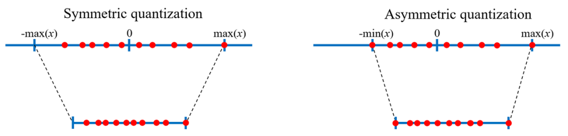
Figure 6-1 Linear Symmetric Quantization and Linear Asymmetric Quantization
6.1.5 Per-Layer Quantization and Per-Channel Quantization
Per-Layer quantization quantizes all channels of a network layer as a whole, and all channels share the same quantization parameters. Per-Channel quantization quantizes individual channels of a network layer independently, and each channel has its own quantization parameters. Per-Channel quantization better preserves the information of each channel, adapts to the differences between different channels, and provides better quantization results.
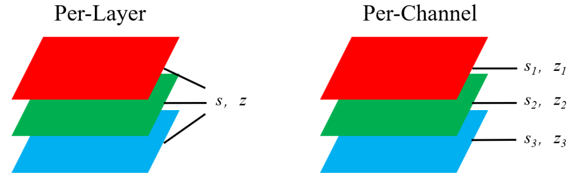
Figure 6-2 Per-Layer Quantization and Per-Channel Quantization
Note: In RKNN-Toolkit2, Per-Channel quantization is only applied to the weights, while the activation values and intermediate values are still quantized using Per-Layer quantization.
6.1.6 Quantization Algorithms
The quantization scale factor and zero point are crucial parameters that affect quantization error, and the solution to the quantization range plays a decisive role in determining the quantization parameters. This section introduces three algorithms for solving the quantization range: Normal, KL-Divergence, and MMSE.
The Normal quantization algorithm determines the maximum and minimum values of the quantization range directly by calculating the maximum and minimum values of the floating-point numbers. From the quantization calculation principle in Chapter 6.1.2, it can be seen that the Normal quantization algorithm does not introduce truncation error but is sensitive to outliers because large outliers may cause significant rounding errors.

q_min = min V

q_max = max V
Where V is the floating-point number tensor.
The KL-Divergence quantization algorithm computes the distributions of the floating-point numbers and fixed- point numbers. It updates the distributions by adjusting different thresholds and determines the maximum and minimum values of the quantization range by minimizing the KL divergence to maximize the similarity between the two distributions. The KL-Divergence quantization algorithm minimizes the distribution difference between the floating-point and fixed-point numbers, allowing it to better adapt to non-uniform data distributions and mitigate the impact of a few outliers.

arg min_(q_min,q_max) H(Ψ(V), Ψ(V_int))
where H(·) is the KL divergence calculation formula, Ψ(·) is the distribution function that discretizes the corresponding data into a discrete distribution, and V_int is the quantized fixed-point number tensor.
The MMSE (Minimum Mean Square Error) quantization algorithm determines the maximum and minimum values of the quantization range by minimizing the mean square error loss between the floating-point numbers and the quantized and dequantized floating-point numbers. It mitigates the quantization accuracy loss caused by large outliers to some extent. The MMSE quantization algorithm is implemented through a brute-force iterative search for an approximate solution, which results in slower speed and higher memory overhead. However, it generally achieves higher quantization accuracy compared to the Normal quantization algorithm.

arg min_(q_min,q_max) ||V - V_hat(q_min, q_max)||_F^2
Where V̂(q_min, q_max) represents the quantized and dequantized form and ‖·‖_F denotes the Frobenius norm.
6.2 Quantization Configuration
6.2.1 Quantization Data Types
RKNN-Toolkit2 supports INT8 as the quantization data type.
6.2.2 Quantization Algorithm Recommendations
The Normal quantization algorithm runs fast and is suitable for general scenarios.
The KL-Divergence quantization algorithm runs slightly slower than the Normal algorithm. It improves quantization accuracy for models with non-uniform distributions and can mitigate quantization accuracy loss caused by a few outlier values.
The MMSE quantization algorithm runs slower and consumes more memory. Compared to the KL-Divergence algorithm, it better mitigates quantization accuracy loss caused by outlier values. For quantization-friendly models, users can try using the MMSE quantization algorithm to improve quantization accuracy. In most scenarios, the MMSE algorithm provides higher quantization accuracy compared to the Normal and KL- Divergence algorithms.
The Normal quantization algorithm is used by default. When encountering quantization accuracy issues, users can try using the KL-Divergence and MMSE quantization algorithms.
6.2.3 Quantization Calibration Set Recommendations
The quantization calibration set is used to compute the quantization range of activation values. When selecting the quantization calibration set, it should cover different data distributions in the actual application scenarios of the model. For example, for a classification model, the quantization calibration set should include images from different categories in the actual application scenario. It is generally recommended to use a quantization calibration set of 20-200 images, which can be adjusted based on the runtime of the quantization algorithm. It should be noted that increasing the number of images in the quantization calibration set will increase the runtime of the quantization algorithm but may not necessarily improve quantization accuracy.
6.2.4 Quantization Configuration Method
The quantization configuration methods in RKNN-Toolkit2 are implemented in the rknn.config() and rknn.build() interfaces. The quantization method configuration is implemented by the rknn.config() interface, and the quantization switch and calibration set path selection are implemented by the rknn.build() interface.
The rknn.config() interface includes the following relevant quantization configuration options:
quantized_dtype: Select the quantization data type. Currently, only linear asymmetric INT8 quantization is supported, and the default value is ‘asymmetric_quantized-8’.
quantized_algorithm: Select the quantization algorithm, including Normal, KL-Divergence, and MMSE quantization algorithms. The optional values are ‘normal’, ‘kl_divergence’, and ‘mmse’, with the default value being ‘normal’.
quantized_method: Select Per-Layer or Per-Channel quantization. The optional values are ‘layer’ and ‘channel’, with the default value being ‘channel’.
The rknn.build() interface includes the following relevant quantization configuration options:
do_quantization: Specify whether to enable quantization, with the default value being ‘False’.
dataset: Specifies the path to the quantization calibration set, with the default value being ‘None’.
Currently, text file format is supported. Users can put the paths of images (in jpg or png format) or npy files for calibration in a .txt file. Each line in the text file represents a path. For example:
a.jpg
b.jpg
If there are multiple inputs, each corresponding file for each input is separated by a space, like this:
a0.jpg a1.jpg
b0.jpg b1.jpg
6.3 Hybrid Quantization
Hybrid quantization applies different quantization data types to different layers of the model. It uses higher precision data types for layers that are not suitable for quantization to mitigate quantization accuracy loss. However, hybrid precision quantization will increase additional overhead and require users to determine the quantization data types for different layers.
6.3.1 Usage of Hybrid Quantization
To achieve a better balance between performance and accuracy, RKNN-Toolkit2 provides a hybrid quantization feature. Users can manually specify whether each layer should be quantized based on the output results of accuracy analysis.
Currently, the hybrid quantization feature supports the following usages:
Changing specified quantized layers to non-quantized layers, using FLOAT16 for computation. (Note that non- quantized computation on the NPU has lower performance, resulting in reduced inference speed.)
The quantization parameters for each layer can also be modified. (It is not recommended to modify the quantization parameters.)
6.3.2 Process of Hybrid Quantization Usage
When using the hybrid quantization feature, it involves four specific steps.
1. Load the original model and generate the quantization configuration file, temporary model file and data file. The specific interface calling process is as follows:
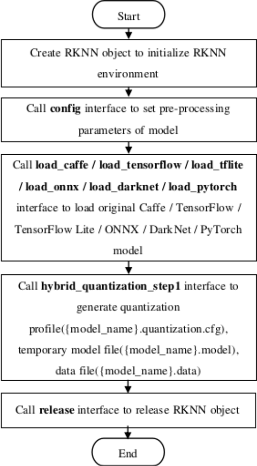
Figure 6-3 Hybrid quantization step 1
2. Modify the quantization configuration file generated in the first step.
After calling the hybrid_quantization_step1 interface in the first step, a configuration file named {model_name}.quantization.cfg will be generated in the current directory. The format of the configuration file is as follows:
custom_quantize_layers:
  Conv__350:0: float16
  Conv__358:0: float16
  ....
quantize_parameters:
  ....
  FeatureExtractor/MobilenetV2/Conv/Relu6:0:
    qtype: asymmetric_quantized
    qmethod: layer
    dtype: int8
    min:
    - 0.0
    max:
    - 6.0
    scale:
    - 0.023529411764705882
    zero_point:
    - -128
  ....
In the “custom_quantize_layers” section, users can add custom quantization layers by specifying the tensor name followed by the quantization type. This will change the operation type of the corresponding layer to the specified type. Currently, the available quantization data type is “float16”.
The “quantize_parameters” section contains the quantization parameters for each tensor in the model. The quantization parameters for each tensor are presented in the format of “tensor_name: quantization_properties_and_parameters”. The “min” and “max” represent the minimum and maximum values of the quantization range. Users can refer to the output results of precision analysis or use Netron to open the temporary model file named {model_name}.model to view the corresponding output tensor names.
3. Generate the RKNN model. The specific interface calling process is as follows:
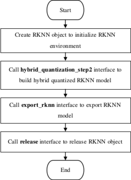
Figure 6-4 Hybrid quantization step 3
4. Perform inference using the RKNN model generated in the third step.
Note: In the RKNN-Toolkit2 project, under the “examples/functions/hybrid_quant” directory, there is an example of hybrid quantization. Users can refer to this example to perform hybrid quantization.
6.3.3 Automatic Hybrid Quantization
To simplify the usage of hybrid quantization and solve model overflow issues, RKNN-Toolkit2 provides an automatic hybrid quantization feature. Users can use the auto_hybrid interface to automatically adjust the hybrid quantization model during model quantization based on Euclidean distance and cosine distance thresholds. For non-quantized models, it will check each layer of the model for fp16 overflow and convert the overflowing layers to int16 computation.
Currently, the automatic hybrid quantization feature supports the following usage scenarios:
1. During model quantization, the hybrid quantization model can be automatically adjusted based on Euclidean distance and cosine distance thresholds. Currently, only automatic adjustment from int8 quantization to fp16 is supported.
ret = rknn.build(do_quantization=True, dataset='./dataset.txt', auto_hybrid=True)
The thresholds for cosine distance and euclidean distance can be configured through using auto_hybrid_cos_thresh and auto_hybrid_euc_thresh in the config interface. The cosine distance default value is 0.98, and the euclidean distance default value is None, meaning it is not enabled. That is, only operators whose cosine distance precision is specified less than the threshold are converted to fp16 by default, and the Euclidean distance threshold is turned off at this time. When the Euclidean distance threshold is turned on, operators lesser than the cosine distance threshold or the greater than euclidean distance threshold are converted to fp16.
2. For non-quantized models, it checks each layer of the model for fp16 overflow and converts the overflowing layers to int16 computation. At this time, you need to provide a dataset to calculate the numerical range of the each layer.
ret = rknn.build(do_quantization=False, dataset='./dataset.txt', auto_hybrid=True)
Calculate the maximum and minimum values layer by layer based on the given input. When the maximum or minimum value exceeds the upper or lower value of fp16, the operator of the corresponding layer will be converted to int16.
6.4 Quantization-Aware Training (QAT)
6.4.1 Introduction to QAT
Quantization-Aware Training (QAT) is a training method aimed at addressing the accuracy loss issue in low-bit quantization. Low-bit quantization can result in accuracy loss because converting the value range from floating- point numbers to fixed-point numbers incurs precision loss. During QAT training, the quantization error is incorporated into the training loss function, allowing the training of a model with quantization parameters.
Contrasting with Post Training Quantization (PTQ) provided by RKNN-Toolkit2, the characteristics of these two quantization methods are as follows:
| Quantization Method |
Secondary training based on the original framework |
Dataset | Adjust the weight parameters |
Loss function | Performance |
|---|---|---|---|---|---|
| Post Training Quantization (PTQ) |
No | Small amount of unlabeled data |
No | Irrelevant | Optimal |
| Quantization- Aware Training (QAT) |
Yes | Complete training dataset |
Yes | Quantization loss is included in the training loss function. |
When there are operators that do not support QAT, the performance is slightly weaker than PTQ. |
6.4.2 QAT Principle
During QAT training, all weights are stored and calculations are performed in floating-point format, which ensures that backpropagation functions properly and the model can be trained effectively. Unlike training a floating-point model, QAT inserts FakeQuantize modules at quantizable locations in the model to simulate precision loss when converting from floating-point numbers to fixed-point numbers. This allows the loss function to recognize and optimize the quantization, ensuring accurate inference results when the model is converted to a fixed-point model.
QAT training is widely used and supported by mainstream inference frameworks. Users can refer to the links below for more detailed usage instructions.
Pytorch - https://pytorch.org/blog/quantization-in-practice/#quantization-aware-training-qat
Paddle - https://paddleslim.readthedocs.io/zh-cn/develop/api_cn/dygraph/quanter/qat.html
Tensorflow - https://www.tensorflow.org/model_optimization/guide/quantization/training
6.4.3 QAT Usage Guidelines
Since using QAT requires additional training code and there may be conflicts with the functionality of some open- source repositories, it is recommended to consider using QAT when both of the following conditions are met:
Refer to Chapter 7 for quantization accuracy investigation to confirm that the PTQ function of RKNN does not meet the accuracy requirements.
Refer to Chapter 6.3 to explore hybrid quantization and confirm that the hybrid quantization function of RKNN does not meet the accuracy and performance requirements.
6.4.4 QAT Implementation Example and Configuration Instructions
Here are the documentations for QAT features in various frameworks. Please refer to the official documentation for actual usage.
PyTorch: https://pytorch.org/docs/stable/quantization.html (PyTorch has multiple sets of quantization interfaces. RKNN currently supports quantized models generated from the FX interface, specifically the prepare_qat_fx interface and its associated interfaces.)
Paddle: https://www.paddlepaddle.org.cn/tutorials/projectdetail/3949129#anchor-14
TensorFlow: https://www.tensorflow.org/model_optimization/guide/quantization/training
Taking PyTorch as an example to demonstrate the process of implementing QAT and some important considerations.
# for 1.10 <= torch <= 1.13
import torch
class M(torch.nn.Module):
 def __init__(self):
 super().__init__()
 self.conv = torch.nn.Conv(3, 8, 3, 1)

 def forward(self, x):
 x = self.conv(x)
 return x

# initialize a floating point model
float_model = M().train()

from torch.quantization import quantize_fx, QConfig, FakeQuantize, MovingAverageMinMaxObserver, MovingAveragePerChannelMinMaxObserver

qconfig = QConfig(activation=FakeQuantize.with_args(observer=
        MovingAverageMinMaxObserver,
        quant_min=0,
        quant_max=255,
        reduce_range=False), # reudece_range -> the default is True

 weight=FakeQuantize.with_args(observer=
      MovingAveragePerChannelMinMaxObserver,
      quant_min=-128,
      quant_max=127,
      dtype=torch.qint8,
      qscheme=torch.per_channel_affine,
      #qscheme->the default is torch.per_channel_symmetric
      reduce_range=False))
qconfig_dict = {"": qconfig}
model_qat = quantize_fx.prepare_qat_fx(float_model, qconfig_dict)

# define the training loop for quantization aware training
def train_loop(model, train_data):
 model.train()
 for image, target in data_loader:
  ...
# Run training
train_loop(model_qat, train_loop)

model_qat = quantize_fx.convert_fx(model_qat)
In the above code flow, except for the adjustments made to the qconfig configuration for RKNN hardware, all other operations are implemented according to the guidance provided in the official codes. There are two main modifications in the qconfig:
The activation quantization configuration specifies reduce_range as False. When reduce_range is False, the effective quantization range is from -128 to 127. When reduce_range is True, the effective quantization range is from -64 to 63, which results in poorer quantization performance. RKNN hardware supports reduce_range as False.
The weight quantization configuration specifies qscheme as torch.per_channel_affine. The default torch.per_channel_symmetric restricts zero_point to be fixed at 0, but RKNN hardware supports non-zero zero_point. Therefore, torch.per_channel_affine is chosen.
6.4.5 Supported Operators in QAT
Taking PyTorch as an example, during the QAT process, Conv and Linear operators with weight parameters are first quantized according to QAT rules. Then other operators are examined. If they meet the regular quantization rules, they will be quantized in regular quantization. If an operator does not meet the QAT and regular quantization rules, it will maintain the FP32 computation rule.
Different frameworks have different levels of support. Users can refer to the following links to find more detailed information about the supported quantization operators based on the framework and version they are using:
Pytorch: https://github.com/pytorch/pytorch/blob/main/torch/ao/quantization/quantization_mappings.py
Paddle: https://github.com/PaddlePaddle/Paddle/blob/86df789a567f1285101c57b6e3ada4b952c58f48/python/pad dle/quantization/config.py
Tensorflow: https://www.tensorflow.org/model_optimization/api_docs/python/tfmot/quantization/keras/QuantizeC onfig
6.4.6 Handling of Floating-Point Operators in QAT Model
In QAT model, when an operator cannot be quantized, floating-point computation will be used. When converting these operators to RKNN models, there are two scenarios to consider.
1. Both preceding and following operators are quantizable:
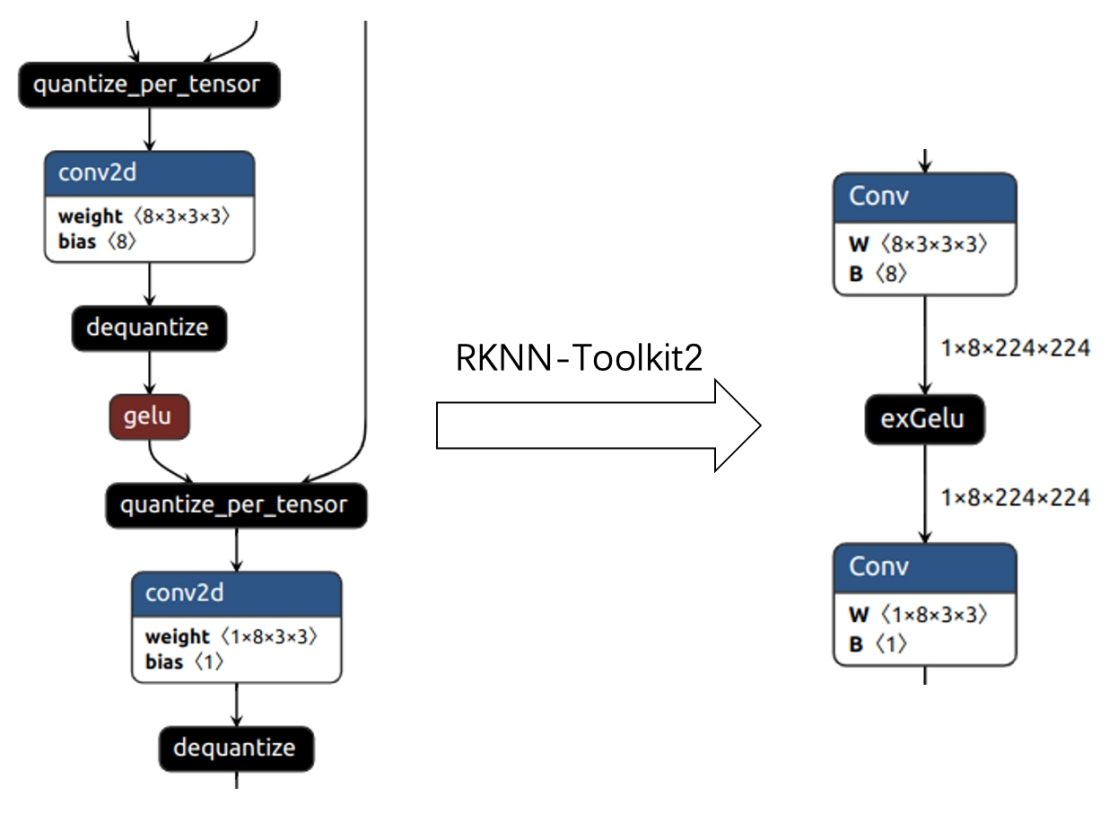
Figure 6-5 QAT OP is preceded and followed by quantifiable operators
As shown in the left image above, the gelu operator in the original model is a floating-point operator, while the preceding and following conv2d operators are quantized. When loading the model with RKNN-Toolkit2, the floating-point operator between the two quantized operators is converted to a quantized operator to improve inference performance without accuracy loss. After conversion to an RKNN model, the structure is as shown in the right image above.
1. Non-quantizable operators exist before or after:
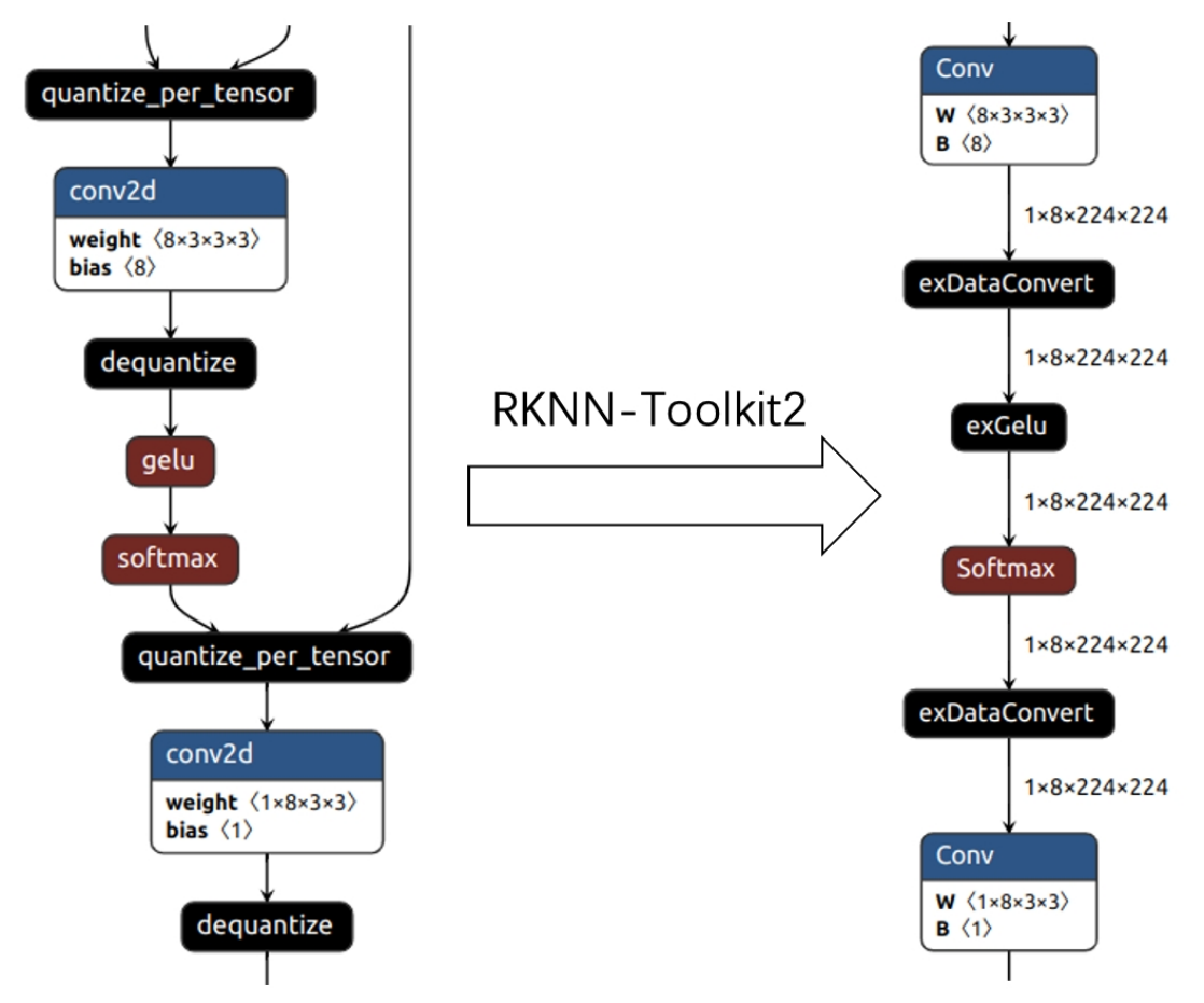
Figure 6-6 QAT OP is preceded and followed by non-quantifiable operators
As shown in the left image above, the gelu and softmax operators in the original model are floating-point operators, while the preceding and following conv2d operators are quantized. When loading the model with RKNN-Toolkit2, since the quantization parameters are missing in gelu and softmax, they will remain in floating- point format. After conversion to an RKNN model, as shown in the right image above, a dequantization operator exDataConvert is inserted before exGelu and a quantization operator exDataConvert is inserted after Softmax. These inserted quantization and dequantization operators will introduce additional latency.
6.4.7 Summary of QAT Experience
1. QAT Configurations
QAT training often requires adjusting the configurations to achieve better results based on the characteristics of different hardware. For RKNPU, it is recommended to refer to the code instructions in Chapter 6.4.4 to configure the qconfig parameters.
2. Adjustment of Saved Quantization Parameters in the Model
For example, in the sigmoid function, the quantization parameters recorded by the sigmoid operator in the model may not be the actual quantization parameters used during inference. In the official code (https://github.com/pytor ch/pytorch/blob/main/aten/src/ATen/native/quantized/cpu/qsigmoid.cpp), the quantization parameters of the sigmoid function are adjusted during inference, setting min to 0 and max to
3. To address this phenomenon, RKNN-Toolkit2 will adjust the quantization parameters for such operators during the model conversion stage to make the inference results closer to the original PyTorch inference results.
7 Accuracy Troubleshooting
The troubleshooting of model accuracy issues generally involves two aspects: simulator accuracy troubleshooting and board-side runtime accuracy troubleshooting. Correct simulator inference results are the prerequisite for correct board-side runtime inference. Therefore, it is essential to prioritize ensuring correct results in the simulator before troubleshooting board-side runtime accuracy issues.
Therefore, this chapter will give troubleshooting suggestions and solutions for simulator accuracy troubleshooting and runtime accuracy troubleshooting. The following figure shows the specific troubleshooting steps:
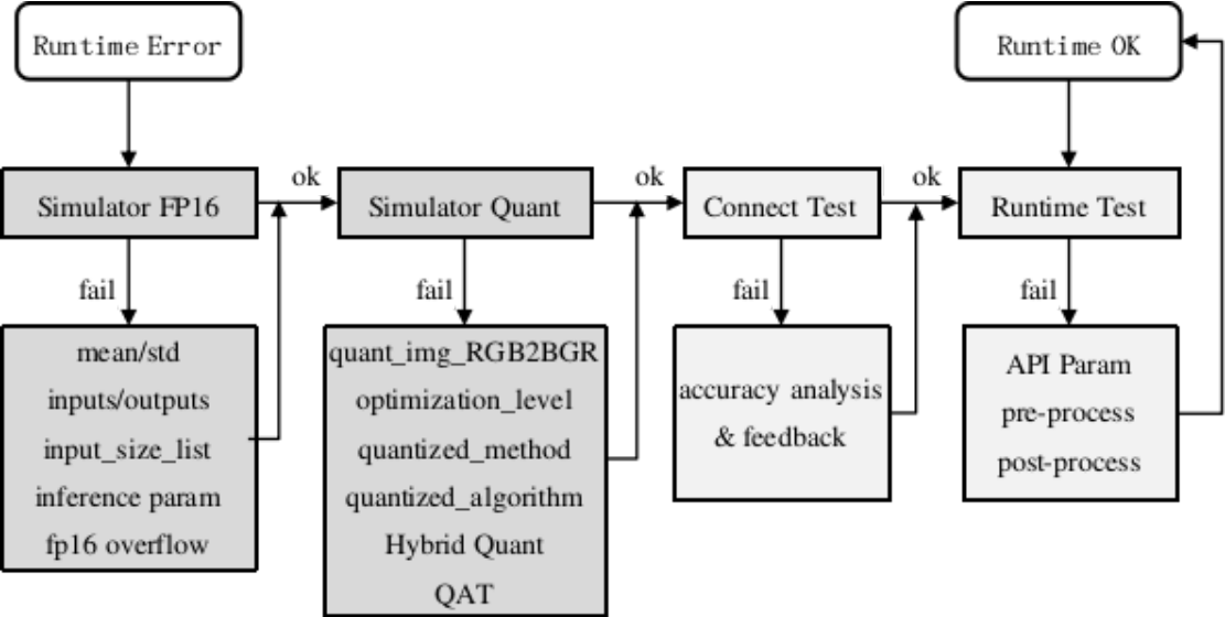
Figure 7-1 The step of accuracy analysis
Simulator accuracy troubleshooting is mainly divided into two sub-steps: simulator FP16 accuracy troubleshooting and simulator quantization accuracy troubleshooting (the dark-colored box in the above figure).
Runtime accuracy troubleshooting is mainly divided into two sub-steps: connecting board accuracy and runtime accuracy troubleshooting (light-colored box in the above figure).
Cosine distance can be used as a basic criterion for judging accuracy, but the final impact of quantization on accuracy still needs validation on the dataset.
7.1 Simulator Accuracy Troubleshooting
Correct simulator inference results are the prerequisite for correct board-side runtime inference, so priority must be given to ensuring that the simulator inference results are correct.
The simulator inference on RKNN-Toolkit2 can be divided into FP16 inference and quantization inference. FP16 inference results must be correct for quantization inference to be correct. Therefore, when there are accuracy issues with quantization inference, it is essential to first verify the correctness of FP16 inference and then troubleshoot the accuracy issues with quantization inference.
7.1.1 Simulator FP16 Accuracy
RKNPU currently does not support FP32 calculations, so the simulator defaults to FP16 computation when quantization is not enabled. To convert the original model to an FP16 RKNN model, use the rknn.build() interface with the do_quantization parameter set False. Then, call rknn.init_runtime(target=None) and rknn.inference()interfaces for FP16 simulation inference and to obtain the output results.
If the FP16 inference output is incorrect, users can perform the following troubleshooting:
Configuration Error
The configuration information of the model is mainly concentrated in the rknn.config() interface. At the same time, there is also a small amount of configuration information in other APIs that may affect the accuracy of FP16. The main parameters are as follows:
mean_values / std_values: Normalization parameters of the model. Generally, the input normalization operation of the original model is implemented in the model’s input preprocessing. However, for RKNN models during inference, this normalization operation can be included (when quantization is enabled, the quantization correction dataset will undergo normalization first). Therefore, when the original model has a normalization step, ensure that these parameters are consistent with the normalization parameters used in the original model.
input_size_list: If the input node shape information of the rknn.load_tensorflow(), rknn.load_pytorch() and rknn.load_onnx() interfaces is configured incorrectly, it will lead to incorrect inference results.
inputs / outputs: If the input and output node names of the rknn.load_tensorflow() and rknn.load_onnx() interfaces are configured incorrectly, it will lead to incorrect inference results.
inference interface parameters: The input parameters for the rknn.inference() interface mainly include inputs and data_format.
Generally in the Python environment, image data is read using cv2.imread(). In this case, it is important to note that the image format read by cv2.imread() is BGR. If the original model’s input is BGR (such as in most caffe models), there is no need to adjust the RGB order. However, if the original model’s input is RGB, users need to use cv2.cvtColor(img, cv2.COLOR_BGR2RGB) to convert the image data to RGB. Additionally, the shape dimensions of the image read by cv2.imread() are 3 dimensions, but the input shape of most models is 4 dimensions. Therefore, users need to use np.expand_dims(img, 0) to expand the input shape to 4 dimensions before passing it to the rknn.inference() interface. The layout of the image read by cv2.imread() is NHWC, and the default value of data_format is also NHWC, so there is no need to set the data_format parameter.
If the model’s input data is not read by cv2.imread(), it is necessary to know the layout of the input data and set the data_format parameter correctly. Also, ensure that the shape of the input data is consistent with the original model. If the input data is image data, ensure that its RGB order is consistent with the original model.
Checking parameter configurations is a crucial step and is the main reason many users encounter incorrect FP16 inference results. The specific troubleshooting steps are as follows:
1. Perform inference using the original model in the original inference framework and save the inference results.
2. Use the RKNN-Toolkit2 to convert and infer the original model. Use the same input data as in the previous step and set the FP16 inference mode (set do_quantization to False in rknn.build()). Also, the target parameter of rknn.init_runtime() is set to None to call the RKNN-Toolkit2 simulator for inference, and save the inference results.
3. Compare the results of the two inferences. If the results are relatively consistent (cosine distance can be used to judge consistency), it indicates that the above configurations are correct.
4. If the results are inconsistent, check whether the above parameters are correct.
If it is confirmed that the above parameter configurations are correct and the results are still inconsistent, it may be due to tensors in the model exceeding the FP16 expression range.
Exceeding the FP16 Expression Range
When converted from FP32 to FP16, the intermediate tensors of the model may encounter overflow issues. Since the typical data type for model inference is FP32, if tensors in the model during inference have values exceeding the FP16 expression range (-65504~65504), the tensor will overflow, resulting in abnormal model inference results.
For overflow issues, users can use the rknn.accuracy_analysis(…, target=None) interface (refer to Model Accuracy Analysis) for simulator FP16 accuracy analysis. If the entire column or single column of simulator_error in the analysis results has an abnormal value (If words such as ‘inf’ appear), an FP16 overflow may occur. In this case, users can try modifying the model structure to ensure that all tensors in the model do not overflow in FP16 (such as adding some BN layers, etc.).
If it is confirmed that the above parameter configurations are correct and there is no FP16 overflow, but the results are still inconsistent, it may be an issue with the internal implementation of the simulator. Please provide the reproduction file of the model to Rockchip NPU team for analysis and resolution.
7.1.2 Simulator Quantization Accuracy
After ruling out FP16 accuracy issues, the model can be quantized (when using the rknn.build() interface, set the do_quantization parameter to True), and then call the rknn.accuracy_analysis(…, target=None) interface (refer to Model Accuracy Analysis) conduct simulator quantization accuracy analysis.
If in the analysis results, users find the accuracy of the entire column of simulator_error has dropped significantly, and there is no specific layer with a considerable decrease in accuracy in the single column of simulator_error, investigate mainly in the following areas:
Configuration Errors
Similar to configuration issues with FP16 inference, incorrect configurations can lead to quantization inference accuracy problems. Therefore, on the basis of ensuring the correct configuration of FP16 inference, the following quantization configuration parameters still need to be checked.
quant_img_RGB2BGR: Indicates whether to perform RGB2BGR operation when loading quantized images, typically used for caffe models. For more detailed information, refer to the explanation of the quant_img_RGB2BGR parameter. This parameter must be consistent with the channel order of the training images. Misconfigurations may lead to a significant decrease in quantization accuracy.
optimization_level: The choice of optimization level, defaulting to 3, representing speed priority. In this case, some optimization rules that slightly affect accuracy are enabled to improve performance. If this configuration is lowered (e.g., set to 0), these optimization rules will be disabled.
dataset: Configuration of the quantization correction dataset for the rknn.build() interface. It is used to calculate appropriate quantization parameters (scale/zero_point) for each tensor during the quantization process. If a correction dataset with significant differences from the actual deployment scenario is selected, it may result in a decrease in accuracy. Additionally, having too many or too few correction set images can affect accuracy (typically choose 20 to 200 images).
To specifically check the quantization parameter configuration issues, generally follow the following steps:
1. Directly perform quantization inference, and then check the inference results and compare them with the inference results of the original model under the original inference framework. If the difference in results is not very large, it can be considered that the quant_img_RGB2BGR and dataset parameters are basically correct.
2. If the difference in results is still obvious:
If the original model’s input image format is BGR (common in caffe models), modify quant_img_RGB2BGR to True. Regarding the RGB order of the model input, users can refer to the input data processing code in the previous FP16 inference accuracy verification step.
Initially, use a single image for quantization (leave only one line in dataset.txt) and perform inference using this image. If the accuracy of a single image improves significantly, it indicates that the previous choice of the quantization correction dataset might not be optimal. Consider reselecting images that better match the deployment scenario (if the improvement is not obvious, it may not be a problem with the dataset).
If only one image was originally used for quantification (there is only one row in dataset.txt), users can try to use more images for quantification, which can be increased to about 20 to 200 images.
After checking the above configuration, there should be no completely wrong quantification results. If there is a completely wrong situation, please recheck the above configuration. After confirming that the configuration is correct, if the accuracy of the model is still not enough, users can try to modify related configurations such as quantization methods and algorithms. Quantization Methods and Quantization Algorithms
Some models are not friendly to quantization. In such cases, try switching to different quantization methods and algorithms. Currently, there are two main quantization methods: layer and channel, which can be set through the quantized_method parameter in the rknn.config() interface (default is channel). Quantization algorithms mainly include normal, kl_divergence, and mmse, which can be set through the quantized_algorithm parameter in the rknn.config() interface (default is normal).Here are the steps:
1. If the original method was layer quantization, try switching to channel quantization. In general, channel quantization often provides significantly higher accuracy than layer quantization.
2. If the quantization method is already channel, but the accuracy is still insufficient, consider changing the quantization algorithm from normal to kl_divergence or mmse. Note that this may significantly increase the quantization time but can yield better accuracy than normal. The runtime performance is not adversely affected.
If after using the above method, the accuracy of the entire column in simulator_error remains unsatisfactory, and some layers in the single column show a significant decrease in accuracy, it may be due to poor weight distribution in these layers, leading to a substantial loss of accuracy after quantization. For example, if the weight distribution of Conv layer weights is highly uneven, users may consider using hybrid quantization to further improve model accuracy. Here are the steps:
1. Use the accuracy analysis interface to analyze the accuracy, find out the layer that causes the accuracy to decrease more, and record the output tensor name of the corresponding layer. (Note: because errors accumulate layer by layer, layers closer to the front have a greater impact on the final accuracy. Therefore, consider both the accuracy loss of the single column of simulator_error and the position of the layer in the model.)
2. Use the hybrid quantization method and write the tensor name obtained in the previous step into the hybrid quantization configuration file (refer to Hybrid Quantization).
3. Complete the steps of hybrid quantification and test the accuracy (users can continue to use the accuracy analysis interface to see the accuracy changes).
Generally, the accuracy of the model can be improved after hybrid quantization. If the improvement is not obvious or not enough, users can try to perform hybrid quantization on more layers. However, this will also cause a decrease in inference performance. Therefore, users need to balance accuracy and speed when applying hybrid quantization. Another special method is that when the Op with reduced accuracy is in the last layer, users can choose to move the execution of that layer’s operation to post-processing, which will also effectively avoid the accuracy problem of this layer.
QAT(Quantization Aware Training):
If the accuracy is still insufficient after hybrid quantization, or if the accuracy is sufficient but the performance does not meet the requirements due to hybrid quantization, users can consider using Quantization-Aware Training (QAT) to retrain the model. Export the model with quantization parameters (e.g., in formats like ONNX, PyTorch, TensorFlow Lite). For more information on Quantization-Aware Training, please refer to Quantization-Aware Training (QAT).
7.2 Runtime Accuracy Troubleshooting
When the accuracy of the simulator is normal, abnormal inference results may still occur when deploying the board-side C API. There are generally three reasons for this problem. The first is caused by a bug in the runtime of the board. The second is incorrect usage of the RKNPU2 C API when programming the interface. The third is incorrect pre-processing or post-processing of the model.
When encountering such problems, users can first use the board-connected function to quickly check whether it is caused by a bug in the runtime of the board. If there are no issues with the board-connected, then check the C API deployment problem.
7.2.1 Board-Connected Accuracy
1. After configuring the board-connected debugging environment (refer to NPU Device Environment Setup for the environment setup), connect the board to the computer via USB, and then use RKNN-Toolkit2 to perform board-connected inference (set the target parameter of rknn.init_runtime(), Such as target=’rk3566’), and check whether the inference results are roughly correct (because the simulator does not strictly simulate NPU hardware, the results may not be completely consistent with the simulator).
2. If the inference results in the above steps are significantly different from the simulator inference results, it can be initially determined that there is a bug in the runtime of the board. In this case, users can use the accuracy analysis interface (refer to Model Accuracy Analysis) to perform board-connected accuracy analysis (use rknn.accuracy_analysis() interface, and set the target parameter, such as target=’rk3566’). After the accuracy analysis is completed, the analysis results of each layer will be output.
3. Check the single_sim column of runtime_error in the analysis results. If its cos cosine distance is low or euc Euclidean distance is high (displayed in yellow or red), resulting in an increasing difference between the entire column of runtime_error and the entire column of simulator_error, it is possible that the runtime has accuracy loss or anomalies when implementing this layer. In this case, the analysis results and reproduced models can be fed back to the Rockchip NPU team for repair.
7.2.2 Runtime Accuracy
If there is no problem with the board-connected accuracy, but there is still a problem with the accuracy, the problem may lie in the C/C++ code itself that the user uses RKNN C API for programming. In this case, the user needs to carefully check whether the interface configuration of RKNN’s C API is configured. Correct, and whether the pre-processing and post-processing processes of the model are correct (they need to be completely consistent with the processes on the simulator side). Users can view it by following these steps:
1. Check Input Configuration and Data
Check whether the input of the C API is configured correctly. For example, RKNN-Toolkit2 has configured the mean and variance when converting the RKNN model, so there is no need to perform normalization in the C/C++ code. For 3-dimensional input, the channel order is consistent with the input channels set during model training; for 4-dimensional input shapes, fmt=NHWC; for non-4-dimensional input, fmt=UNDEFINED. If users use the general API, the size of the input buffer is equal to the number of input tensor elements * the number of bytes of each element. If users use the zero-copy API, please refer to the “RKNN Runtime Zero-Copy Usage” chapter for the memory size and input data format created by the rknn_create_mem interface.
After confirming that the configuration is correct, users need to check the data of the input layer. users can set RKNN_LOG_LEVEL=5 before running the application. The layer-by-layer results during inference will be saved in numpy format files in /data/dumps (Android system) or /userdata/dumps (Linux system) directory. Check whether the numpy file containing the InputOperator field meets expectations. If users use the general API, it is the result of input normalization; if users use the zero-copy API, it is the data before normalization.
2. Check Output Configuration and Data
After ensuring that the input is correct, check whether the output in the code is configured correctly. For example, if users use the general API, when setting want_float=1, the output is a float32 type result. When setting want_float=0, the output is a quantized data type or FP16 type (non-quantified data type). If users use the zero-copy API, please refer to the “RKNN Runtime Zero-Copy Usage” chapter for the memory size and input data format created by the rknn_create_mem() interface.
Check the data of the output layer. Similarly, after the above layer-by-layer numpy files are generated, open the numpy file containing the OutputOperator field to check whether the data is correct. If the input results are confirmed correctly but the output is still wrong, there may be a problem with the specific input/output type processing in runtime. In this case, the analysis results and the reproduced model can be fed back to the Rockchip NPU team for repair.
8 Performance optimization
8.1 Process of Model Performance Optimization Analysis
8.1.1 Checking the Runtime Environment
At the beginning of all performance analysis and optimization, it is important to establish a baseline for the test environment. Only when the baselines are the same, the measured performance data becomes meaningful. For example, testing the inference performance of the same model under different frequencies can result in significant fluctuations and can not be represented by the average frame time of a single batch.
There are several aspects to consider when querying and configuring the test environment:
Querying and setting CPU, DDR, and NPU frequencies
Fixed frequencies directly impact the execution speed, where higher frequencies generally yield better performance. However, the relationship between frequency changes and performance improvement is not linear. Increasing the frequency also leads to increased power consumption.
You can refer to the command for setting fixed frequencies: https://github.com/airockchip/rknn_model_zoo/ blob/main/scaling_frequency.sh
Alternatively, you can use the following command to set the performance mode:
echo performance | tee $(find /sys/ -name *governor) /dev/null || true
Checking the NPU kernel driver version
The performance optimization options for certain features or operators may be specific to the kernel driver version. Newer kernel driver versions can incorporate the latest underlying optimization implementations. Therefore, please check if you are using a relatively recent kernel driver version. It is recommended to update to version 0.8.8 or later. This step is not mandatory.
You can check the kernel driver version using the following commands:
cat /sys/kernel/debug/rknpu/version # for RK3566/RK3568/RK3588/RK3562/RK3576
cat /proc/rknpu/version # for RV1106/RV1106B/RV1103/RV1103B/RV1126B
Note: RK2118 does not support checking NPU version number yet. Checking the NPU load
The NPU load represents the percentage of time the NPU is executing tasks within a unit of time. The load reflects the level of NPU activity. If the queried load is low, it indicates that the NPU is waiting for task submissions for a longer duration. In such cases, it is necessary to investigate factors such as data input/output copy time, preprocessing and post-processing optimizations in the application, etc. Alternatively, utilizing multi-threading in the application can help increase the NPU load.
It is important to note that the NPU load does not directly represent the actual MAC utilization. MAC utilization reflects the efficiency of task execution in the NPU hardware unit.
The command to query the NPU load is as follows:
cat /sys/kernel/debug/rknpu/load
# or
cat /proc/debug/rknpu/load
Note: RK2118 does not support checking NPU load yet.
8.1.2 Deployment Time Analysis
The entire deployment process can be divided into three aspects in terms of time consumption: user application time, input-output data copy time, and model inference time. Analyzing the time distribution of each step can help identify optimization priorities. The time consumption of these steps can be measured by timestamping in the application.
User application time:
User application time mainly refers to the non-NPU-related time during the inference process. Typically, it includes pre-processing, post-processing, and the execution time of logical code. Users have full control over this part. If the application time is significantly high in proportion to the overall time, besides optimizing and simplifying the code, user can try to accelerate some operations using dedicated hardware.
For example, matrix multiplication and addition operations can be accelerated by using the Matmul API to invoke NPU-assisted computation. Similarly, image scaling operations can be accelerated by invoking the interfaces of RGA.
Input-output copy time:
When using the general API, there is a copy time involved between the input/output memory and the NPU memory. This time can be printed when calling the general API. The copy time depends on the performance of DDR and CPU. When the input-output data is small, the copy time is low. However, when the data is large, it’s time can’t be ignored. Therefore, it is recommended to use zero-copy APIs.
When using zero-copy APIs, the input-output memory is directly accessed by the NPU. For detailed usage of zero-copy interfaces, please refer to RKNN Runtime Zero-Copy Interface.
Inference time:
The time consumed by the NPU for inference is influenced by factors such as the size of the model and the version of the compiler optimization. The reasoning time of RKNN’s LOG printing is different at different RKNN_LOG_LEVEL levels because LOG printing takes a certain amount of time.
Generally, when viewing the time taken for single-frame inference, the LOG level is set to 1, and the average is taken after running multiple times.
8.2 Performance Analysis
8.2.1 Obtain Profile information
When you need to know the time consumption of model inference layer by layer, you can enter the following command to print detailed information before running the program:
export RKNN_LOG_LEVEL=4
./run_rknn_test ./test.rknn ./input.jpg
If it is on the Android platform, you can obtain detailed logs through the logcat command after running.
If you are using RKNN-Toolkit2, you can use the following method to get the time consumption of each layer.
rknn.init_runtime(target=platform, perf_debug=True)
rknn.eval_perf()
You can get the following performance analysis report:
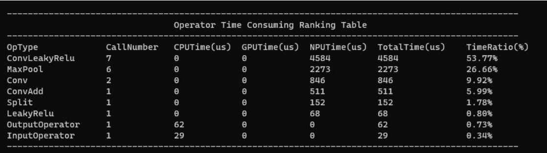
| OpType | CallNumber | CPUTime(us) | GPUTime(us) | NPUTime(us) | TotalTime(us) | TimeRatio(%) |
|---|---|---|---|---|---|---|
| ConvLeakyRelu | 7 | 0 | 0 | 4584 | 4584 | 53.77% |
| MaxPool | 6 | 0 | 0 | 2273 | 2273 | 26.66% |
| Conv | 2 | 0 | 0 | 846 | 846 | 9.92% |
| ConvAdd | 1 | 0 | 0 | 511 | 511 | 5.99% |
| Split | 1 | 0 | 0 | 152 | 152 | 1.78% |
| LeakyRelu | 1 | 0 | 0 | 68 | 68 | 0.80% |
| OutputOperator | 1 | 62 | 0 | 0 | 62 | 0.73% |
| InputOperator | 1 | 29 | 0 | 0 | 29 | 0.34% |
Figure 8-1 Performance analysis report
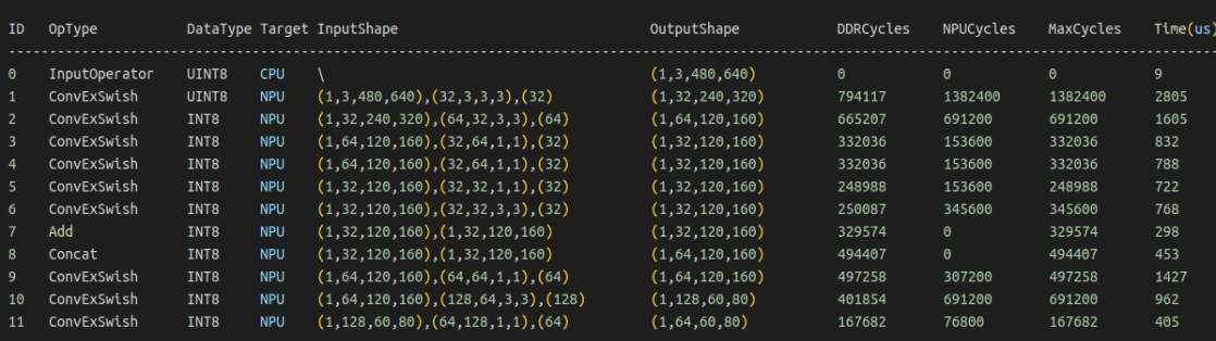
| ID | OpType | DataType | Target | InputShape | OutputShape | DDRCycles | NPUCycles | MaxCycles | Time(us) |
|---|---|---|---|---|---|---|---|---|---|
| 0 | InputOperator | UINT8 | CPU | \ | (1,3,480,640) | 0 | 0 | 0 | 9 |
| 1 | ConvExSwish | INT8 | NPU | (1,3,480,640),(32,3,3,3),(32) | (1,32,240,320) | 794117 | 1382400 | 1382400 | 2805 |
| 2 | ConvExSwish | INT8 | NPU | (1,32,240,320),(64,32,3,3),(64) | (1,64,120,160) | 665207 | 691200 | 691200 | 1605 |
| 3 | ConvExSwish | INT8 | NPU | (1,64,120,160),(32,64,1,1),(32) | (1,32,120,160) | 332036 | 153600 | 332036 | 832 |
| 4 | ConvExSwish | INT8 | NPU | (1,64,120,160),(32,64,1,1),(32) | (1,32,120,160) | 332036 | 153600 | 332036 | 788 |
| 5 | ConvExSwish | INT8 | NPU | (1,32,120,160),(32,32,1,1),(32) | (1,32,120,160) | 248988 | 153600 | 248988 | 722 |
| 6 | ConvExSwish | INT8 | NPU | (1,32,120,160),(32,32,3,3),(32) | (1,32,120,160) | 250087 | 345600 | 345600 | 768 |
| 7 | Add | INT8 | NPU | (1,32,120,160),(1,32,120,160) | (1,32,120,160) | 329574 | 0 | 329574 | 298 |
| 8 | Concat | INT8 | NPU | (1,32,120,160),(1,32,120,160) | (1,64,120,160) | 494407 | 0 | 494407 | 453 |
| 9 | ConvExSwish | INT8 | NPU | (1,64,120,160),(64,64,1,1),(64) | (1,64,120,160) | 497258 | 307200 | 497258 | 1427 |
| 10 | ConvExSwish | INT8 | NPU | (1,64,120,160),(128,64,3,3),(128) | (1,128,60,80) | 401859 | 691200 | 691200 | 962 |
| 11 | ConvExSwish | INT8 | NPU | (1,128,60,80),(64,128,1,1),(64) | (1,64,60,80) | 167682 | 76800 | 167682 | 405 |
Figure 8-2 Performance analysis report
You can quickly locate the desired information based on the overall performance profile and layer-by-layer performance profile. Based on the data, we can formulate subsequent optimization strategies with different focuses. After obtaining the Profile, you can perform the following analysis: analyze the time consumption layer by layer to find out the high time-consuming operators; analyze the impact of non-NPU operators; analyze the performance bottleneck of NPU operators. This is discussed in detail below.
8.2.2 Analyzing the time-consuming layer by layer
As shown in the figure below, you can find the operators with high time consumption from the Times column and optimize the operators with high time consumption first. You can also look at the Op Type column to find out whether the highly time-consuming operators belong to the same OpType, so that they can be optimized uniformly.
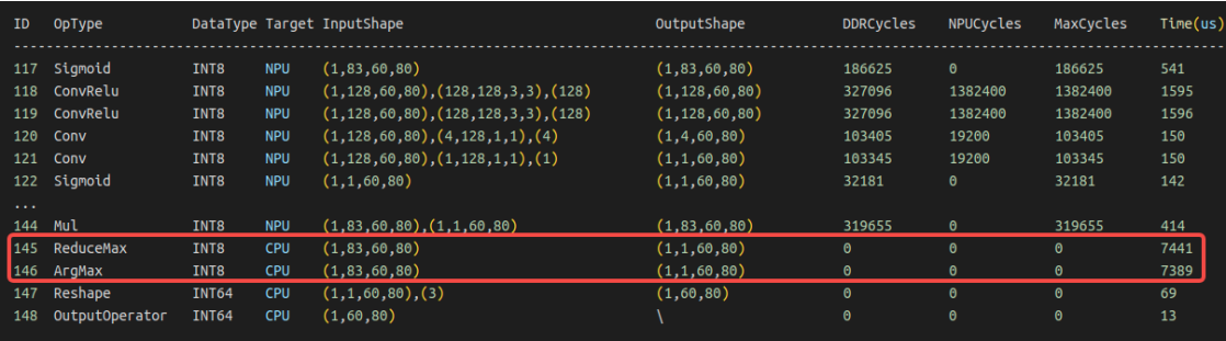
| ID | OpType | DataType | Target | InputShape | OutputShape | DDRCycles | NPUCycles | MaxCycles | Time(us) |
|---|---|---|---|---|---|---|---|---|---|
| 117 | Sigmoid | INT8 | NPU | (1,83,60,80) | (1,83,60,80) | 186625 | 0 | 186625 | 541 |
| 118 | ConvRelu | INT8 | NPU | (1,128,60,80),(128,128,3,3),(128) | (1,128,60,80) | 327096 | 1382400 | 1382400 | 1595 |
| 119 | ConvRelu | INT8 | NPU | (1,128,60,80),(128,128,3,3),(128) | (1,128,60,80) | 327096 | 1382400 | 1382400 | 1596 |
| 120 | Conv | INT8 | NPU | (1,128,60,80),(4,128,1,1),(4) | (1,4,60,80) | 103405 | 19200 | 103405 | 150 |
| 121 | Conv | INT8 | NPU | (1,128,60,80),(1,128,1,1),(1) | (1,1,60,80) | 103345 | 19200 | 103345 | 150 |
| 122 | Sigmoid | INT8 | NPU | (1,1,60,80) | (1,1,60,80) | 32181 | 0 | 32181 | 142 |
| … | … | … | … | … | … | … | … | … | … |
| 144 | Mul | INT8 | NPU | (1,83,60,80),(1,1,60,80) | (1,83,60,80) | 319655 | 0 | 319655 | 414 |
| 145 | ReduceMax | INT8 | CPU | (1,83,60,80) | (1,1,60,80) | 0 | 0 | 0 | 7441 |
| 146 | ArgMax | INT8 | CPU | (1,83,60,80) | (1,1,60,80) | 0 | 0 | 0 | 7389 |
| 147 | Reshape | INT64 | CPU | (1,1,60,80),(3) | (1,60,80) | 0 | 0 | 0 | 69 |
| 148 | OutputOperator | INT64 | CPU | (1,60,80) | \ | 0 | 0 | 0 | 13 |
Figure 8-3 Performance analysis of time-consuming operators
A time-consuming operator is not necessarily an inefficient operator. If its Mac utilization is high, you should consider reducing the size of the operator to reduce time consumption. But when utilization is low, focus is needed.
8.2.3 Analyze the impact of CPU operators
As shown in the figure below, you can see that some time-consuming operators run on the CPU. Converting these CPU operators to NPU can greatly improve the impact of high time-consuming operations. Most of the performance optimization problems of users will be solved after converting the CPU operators to NPU. Therefore, we should pay special attention to the time-consuming situation of CPU operators.
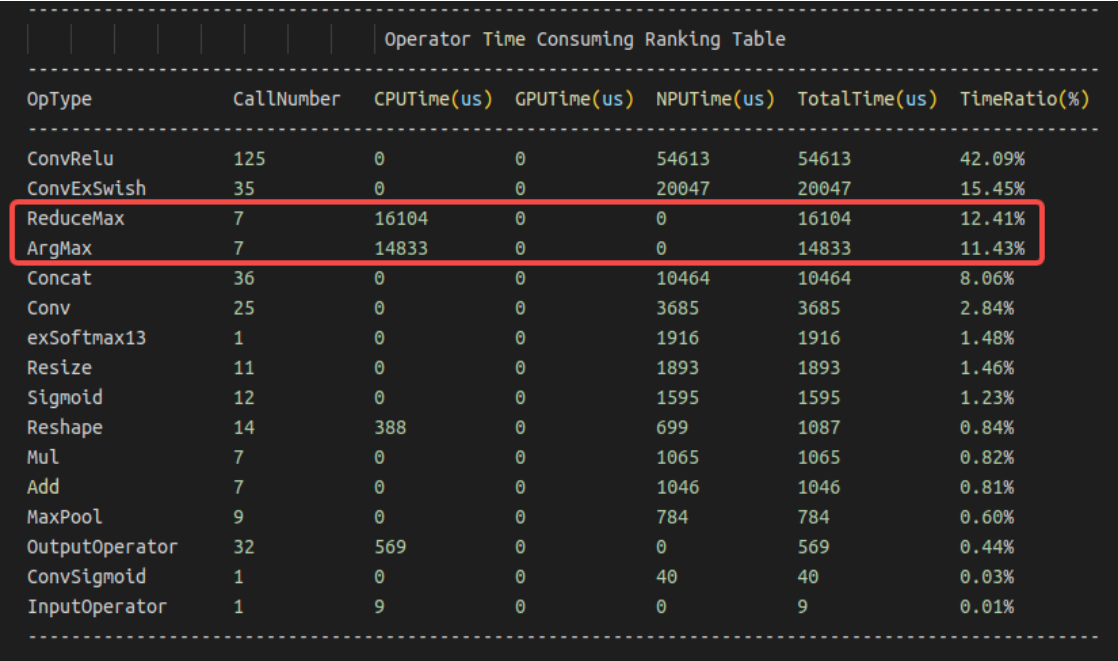
| OpType | CallNumber | CPUTime(us) | GPUTime(us) | NPUTime(us) | TotalTime(us) | TimeRatio(%) |
|---|---|---|---|---|---|---|
| ConvRelu | 125 | 0 | 0 | 54613 | 54613 | 42.09% |
| ConvExSwish | 35 | 0 | 0 | 20047 | 20047 | 15.45% |
| ReduceMax | 7 | 16104 | 0 | 0 | 16104 | 12.41% |
| ArgMax | 7 | 14833 | 0 | 0 | 14833 | 11.43% |
| Concat | 36 | 0 | 0 | 10464 | 10464 | 8.06% |
| Conv | 25 | 0 | 0 | 3685 | 3685 | 2.84% |
| exSoftmax13 | 1 | 0 | 0 | 1916 | 1916 | 1.48% |
| Resize | 11 | 0 | 0 | 1893 | 1893 | 1.46% |
| Sigmoid | 12 | 0 | 0 | 1595 | 1595 | 1.23% |
| Reshape | 14 | 388 | 0 | 699 | 1087 | 0.84% |
| Mul | 7 | 0 | 0 | 1065 | 1065 | 0.82% |
| Add | 7 | 0 | 0 | 1046 | 1046 | 0.81% |
| MaxPool | 9 | 0 | 0 | 784 | 784 | 0.60% |
| OutputOperator | 32 | 569 | 0 | 0 | 569 | 0.44% |
| ConvSigmoid | 1 | 0 | 0 | 40 | 40 | 0.03% |
| InputOperator | 1 | 9 | 0 | 0 | 9 | 0.01% |
Figure 8-4 CPU operator performance analysis
Generally speaking, the reasons why operators run on non-NPU are as follows:
The operator size exceeds the limit (see the operator size limit in the OpList document)
The operator does not yet support operation on NPU (check whether OpList supports this operator, you can submit an issue on the Github project)
NPU hardware limitations cannot support it (can the algorithm be equivalent to other implementations supported by other NPUs)
8.2.4 Analysis of NPU operator performance bottlenecks
When analyzing the high time-consuming problem of the NPU operator, you can judge whether the theoretical bottleneck of the operator’s time-consuming is a bandwidth bottleneck or a computing power bottleneck based on the three columns of DDR Cycles/NPU Cycles/Total Cycles. DDR Cycles refers to the number of cycles required by the operator to read and write. It has been converted into the number of Cycles required at the NPU frequency, so it can be directly compared with the NPU Cycle.
As shown below:
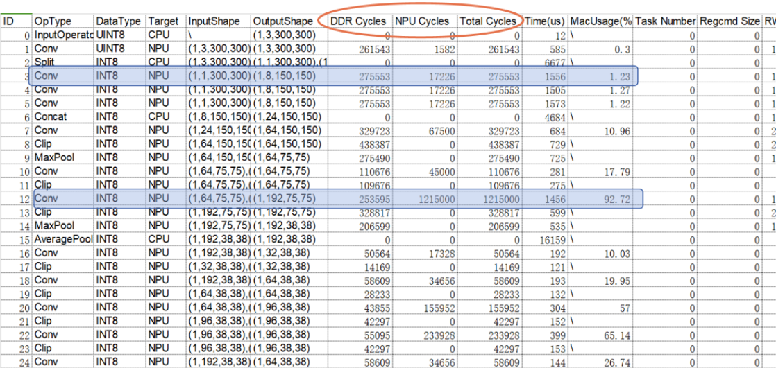
| ID | OpType | DataType | Target | InputShape | OutputShape | DDR Cycles | NPU Cycles | Total Cycles | Time(us) | MacUsage(% [clipped] | Task Number | Regcmd Size | RW [clipped] |
|---|---|---|---|---|---|---|---|---|---|---|---|---|---|
| 0 | InputOperat [clipped] | UINT8 | CPU | \ | (1,3,300,300) | 0 | 0 | 0 | 12 | \ | 0 | 0 | [clipped] |
| 1 | Conv | UINT8 | NPU | (1,3,300,300) | (1,3,300,300) | 261543 | 1582 | 261543 | 585 | 0.3 | 0 | 0 | 1 [clipped] |
| 2 | Split | INT8 | CPU | (1,3,300,300) | (1,1,300,300),(1 [clipped] | 0 | 0 | 0 | 6677 | \ | 0 | 0 | [clipped] |
| 3 | Conv | INT8 | NPU | (1,1,300,300) | (1,8,150,150) | 275553 | 17226 | 275553 | 1556 | 1.23 | 0 | 0 | 1 [clipped] |
| 4 | Conv | INT8 | NPU | (1,1,300,300) | (1,8,150,150) | 275553 | 17226 | 275553 | 1505 | 1.27 | 0 | 0 | 1 [clipped] |
| 5 | Conv | INT8 | NPU | (1,1,300,300) | (1,8,150,150) | 275553 | 17226 | 275553 | 1573 | 1.22 | 0 | 0 | 1 [clipped] |
| 6 | Concat | INT8 | CPU | (1,8,150,150) [clipped] | (1,24,150,150) | 0 | 0 | 0 | 4684 | \ | 0 | 0 | 1 [clipped] |
| 7 | Conv | INT8 | NPU | (1,24,150,150) | (1,64,150,150) | 329723 | 67500 | 329723 | 684 | 10.96 | 0 | 0 | 2 [clipped] |
| 8 | Clip | INT8 | NPU | (1,64,150,150) | (1,64,150,150) | 438387 | 0 | 438387 | 729 | \ | 0 | 0 | 2 [clipped] |
| 9 | MaxPool | INT8 | NPU | (1,64,150,150) | (1,64,75,75) | 275490 | 0 | 275490 | 725 | \ | 0 | 0 | 1 [clipped] |
| 10 | Conv | INT8 | NPU | (1,64,75,75) | (1,64,75,75) | 110676 | 45000 | 110676 | 281 | 17.79 | 0 | 0 | [clipped] |
| 11 | Clip | INT8 | NPU | (1,64,75,75) | (1,64,75,75) | 109676 | 0 | 109676 | 275 | \ | 0 | 0 | [clipped] |
| 12 | Conv | INT8 | NPU | (1,64,75,75) | (1,192,75,75) | 253595 | 1215000 | 1215000 | 1456 | 92.72 | 0 | 0 | 1 [clipped] |
| 13 | Clip | INT8 | NPU | (1,192,75,75) | (1,192,75,75) | 328817 | 0 | 328817 | 599 | \ | 0 | 0 | 2 [clipped] |
| 14 | MaxPool | INT8 | NPU | (1,192,75,75) | (1,192,38,38) | 206599 | 0 | 206599 | 535 | \ | 0 | 0 | 1 [clipped] |
| 15 | AveragePool [clipped] | INT8 | CPU | (1,192,38,38) | (1,192,38,38) | 0 | 0 | 0 | 16159 | \ | 0 | 0 | [clipped] |
| 16 | Conv | INT8 | NPU | (1,192,38,38) | (1,32,38,38) | 50564 | 17328 | 50564 | 192 | 10.03 | 0 | 0 | [clipped] |
| 17 | Clip | INT8 | NPU | (1,32,38,38) | (1,32,38,38) | 14169 | 0 | 14169 | 121 | \ | 0 | 0 | [clipped] |
| 18 | Conv | INT8 | NPU | (1,192,38,38) | (1,64,38,38) | 58609 | 34656 | 58609 | 139 | 19.95 | 0 | 0 | [clipped] |
| 19 | Clip | INT8 | NPU | (1,64,38,38) | (1,64,38,38) | 28233 | 0 | 28233 | 132 | \ | 0 | 0 | [clipped] |
| 20 | Conv | INT8 | NPU | (1,64,38,38) | (1,96,38,38) | 43855 | 155952 | 155952 | 304 | 57 | 0 | 0 | [clipped] |
| 21 | Clip | INT8 | NPU | (1,96,38,38) | (1,96,38,38) | 42297 | 0 | 42297 | 152 | \ | 0 | 0 | [clipped] |
| 22 | Conv | INT8 | NPU | (1,96,38,38) | (1,96,38,38) | 55095 | 233928 | 233928 | 399 | 65.14 | 0 | 0 | [clipped] |
| 23 | Clip | INT8 | NPU | (1,96,38,38) | (1,96,38,38) | 42297 | 0 | 42297 | 153 | \ | 0 | 0 | [clipped] |
| 24 | Conv | INT8 | NPU | (1,192,38,38) | (1,64,38,38) | 58609 | 34656 | 58609 | 144 | 26.74 | 0 | 0 | [clipped] |
Figure 8-5 NPU operator performance analysis
For third layer, DDR Cycles are much larger than the NPU Cycles, it means that the number of Cycles consumed by this layer to read and write data is much greater than the number of Cycles required for operation, so the Conv bottleneck comes from bandwidth.
For twelfth layer, DDR Cycles are much smaller than the NPU Cycles, it means that the number of Cycles required for reading and writing data in this layer is much less than the number of Cycles required for operation, so the Conv bottleneck comes from calculation.
Currently, the NPU Cycles column only displays the Cycles required by Conv, and other operator types will be added later.
8.3 Quantitative acceleration
Quantization can significantly reduce the calculation amount of the model and save bandwidth consumption. On the other hand, the INT8 computing power of NPU is much greater than that of FP16, so quantization can greatly improve the model running speed. We recommend using quantitative model deployment. For details on how to use model quantification, see Introduction to Quantization.
8.4 Graph optimization
Graph optimization of the model is the easiest way to coordinate and optimize the model from an overall perspective. After analyzing the operators or subgraphs that take a high proportion of time, we can transform the graph in many different ways to achieve optimization. Graph optimization mainly aims at saving redundant operators, converting non-NPU OPs into NPUs, and transforming hardware-oriented high-efficiency operators. These goals may sometimes be contradictory. For example, in order to convert non-NPU OP to NPU, a few additional operators may be needed. This may seem to violate the goal of saving redundant operators, but the overall inference performance improvement is beneficial. meaningful.
In the RKNN-Toolkit2 toolchain, the software stack already performs graph optimization to a certain extent during the model conversion process. However, this process is not omnipotent and perfect. Some scenarios that have not been considered will still have redundant operations. Users can perform pre-emptive graph optimization based on some of the ideas introduced in this section. The following is only an introduction to each optimization method. It is not mandatory and needs to be used flexibly in actual scenarios.
8.4.1 Convert non-NPU OP to NPU OP
For non-NPU ops, you can do some equivalent graph transformations and replace them with operators that can be supported by NPU to achieve NPU optimization.
For example, in the figure below, the shufflenetv2_0.5 model is taken as an example, and the channel shuffle operation is changed to convolution approximate replacement. The weight value is 0/1, which can achieve the effect of data rearrangement. If the Transpose and Reshape operations cannot be implemented on the NPU, these operators can be integrated into the Conv operator to achieve data rearrangement.
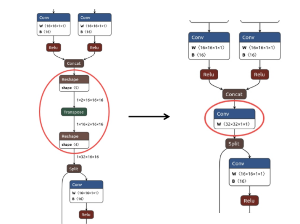
Figure 8-6 Convolution rearrangement
8.4.2 Use hardware Fuse feature to design network or graph optimization
NPU supports fusion of some operators, and the operation process of some operators can be appropriately adjusted to adapt to the fusion rules of NPU.
Although the RKNN software stack will have a certain degree of graph optimization, it cannot fully cover all situations. In some special cases, there are graph structures that can be theoretically fused, but fail to be fused in the final graph optimization. Users can manually adjust the algorithm to solve the problem.
For example, in the figure below, without changing the correctness of the calculation, by adjusting the order of the Transpose and Clip operators, the Conv and Clip fusion operations are performed, improving performance.
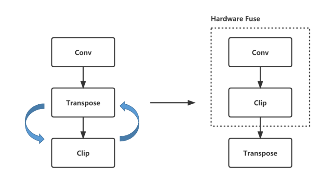
Figure 8-7 Operator graph optimization/fusion
The hardware fusion rules are as follows:
| Supported fusion rules | Fusion rules supported by future plans |
|---|---|
| Conv+Relu | Activation+Add(Mul) |
| Conv+PRelu(LeakyRelu) | Add(Mul)+Activation |
| Conv+Clip | Conv+Mul |
| Conv+Sigmoid(Tanh/Elu/Silu…) | Conv+Activation+Mul |
| Conv+Add | Conv+Activation+Pooling |
| Conv+Activation+Add | Conv+Activation+Add(Mul)+Pooling |
8.4.3 Subgraph transformation
When analyzing a certain subgraph, sometimes the algorithm does not consider the performance impact of specific deployment in order to be intuitive, and it is easy to produce a complex and redundant graph structure. The subgraph in a certain area can be optimized through algorithmic equivalence. Reduce operator calculation steps.
For example, the figure below shows the Yolov5-nano equivalent graph transformation, which integrates several complex Slice numbers into Conv to form a new Conv, which greatly simplifies the graph structure.
Solution source: https://github.com/ultralytics/yolov5/issues/4825
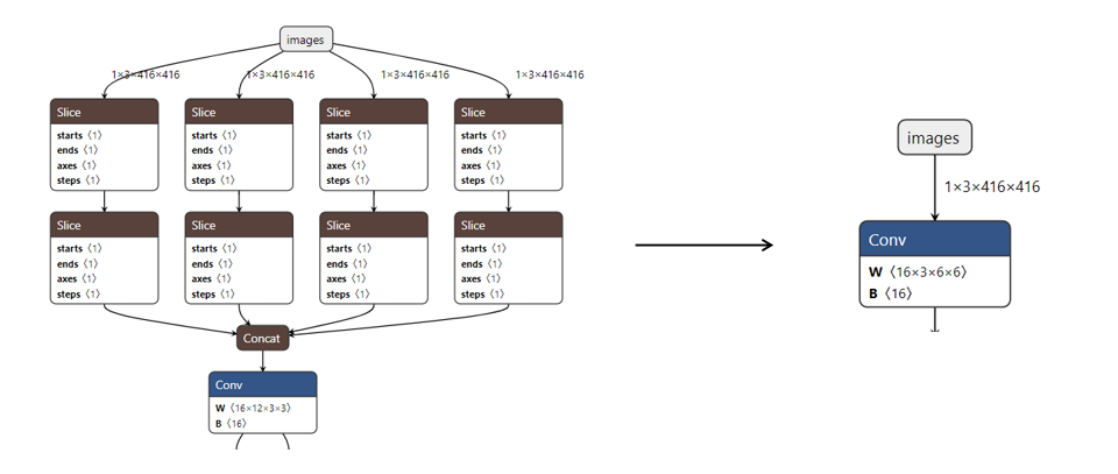
Figure 8-8 Operator equivalent graph transformation
8.4.4 “Combining similar terms” and “Extracting common factors”
When certain operators are operated multiple times in succession, they can be simply merged into the same operator, such as Reshape, Transpose, Slice, some Add/Mul/Sub/Div, etc.
For example, in the figure below, similar operators can be merged by simply adjusting the order of the figures.
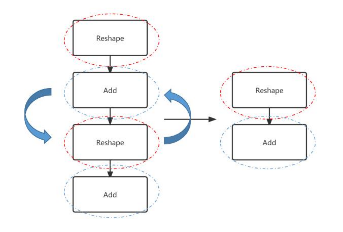
Figure 8-9 Operator merging of similar terms
Some graph structures have some common parts where operations of the same type can be reordered to extract them into a single operation.
For example, in the figure below, the reshape operator can be extracted separately by adjusting the operator order to perform only one operation.
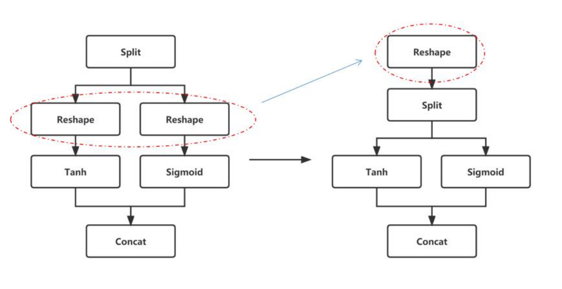
Figure 8-10 Repeatability operator merging
8.5 Operator level optimization
The operator-level optimization of the model is a relatively targeted optimization, and the specific transformation design of some specific operators can further improve performance. Optimization of operators is more about targeted operator size design and running with the most efficient size specifications for hardware implementation. For example, some operators are similar in size and scale, and the running time of aligned and non-aligned operations may be very different. The reason for the difference is Hardware will require additional redundant operations to ensure correctness for some non-aligned size operators. Therefore, the size design of the operator can also have a great impact on model performance. Users can optimize the operator according to the following ideas:
8.5.1 DDR-friendly OP size design (not mandatory)
Under some alignment sizes, in addition to higher NPU computing efficiency, it is also more friendly to DDR reading and writing. Under the same bandwidth conditions, more friendly reading and writing will improve the bandwidth efficiency of DDR, thereby achieving better performance. Listed below are some size rules that are more friendly to DDR reading and writing. These rules are not mandatory.
Channel alignment requirements
Alignment requirements are shown in the table below
Table 8-1 RK3566/RK3568
| Conv | Depthwise Conv | Other OP | ||
|---|---|---|---|---|
| Dtype | Input Channel |
Output Channel |
Input & Output Channel |
Input & Output Channel |
| Int8 | 32 | 16 | 32 | 8 |
| Int16 | 16 | 8 | 16 | 4 |
| Float16 | 16 | 8 | 16 | 4 |
| BFloat16 | 16 | 8 | 16 | 4 |
Table 8-2 RK3588/RK3576/RV1126B
| Conv | Depthwise Conv | Other OP | ||
|---|---|---|---|---|
| Dtype | Input Channel |
Output Channel |
Input & Output Channel |
Input & Output Channel |
| Int8 | 32 | 32 | 64 | 16 |
| Int16 | 32 | 16 | 32 | 8 |
| Float16 | 32 | 16 | 32 | 8 |
| BFloat16 | 32 | 16 | 32 | 8 |
| TFloat32 | 16 | 16 | 16 | 4 |
Table 8-3 RV1106/RV1103
| Conv | Depthwise Conv | Other OP | ||
|---|---|---|---|---|
| Dtype | Input Channel |
Output Channel |
Input & Output Channel |
Input & Output Channel |
| Int8 | 32 | 16 | 32 | 16 |
| Int16 | 16 | 16 | 16 | 8 |
Table 8-4 RK3562
| Conv | Depthwise Conv | Other OP | ||
|---|---|---|---|---|
| Dtype | Input Channel |
Output Channel |
Input & Output Channel |
Input & Output Channel |
| Int8 | 32 | 16 | 32 | 16 |
| Int16 | 32 | 8 | 16 | 8 |
| Float16 | 32 | 8 | 16 | 8 |
| BFloat16 | 32 | 8 | 16 | 8 |
| TFloat32 | 16 | 8 | 8 | 4 |
4 aligned when Height * Width > 1
Operators of the same size have larger Width and smaller Height, making them more friendly for DDR reading and writing. As shown below: The convolution efficiency of the right image is higher than that of the left image.
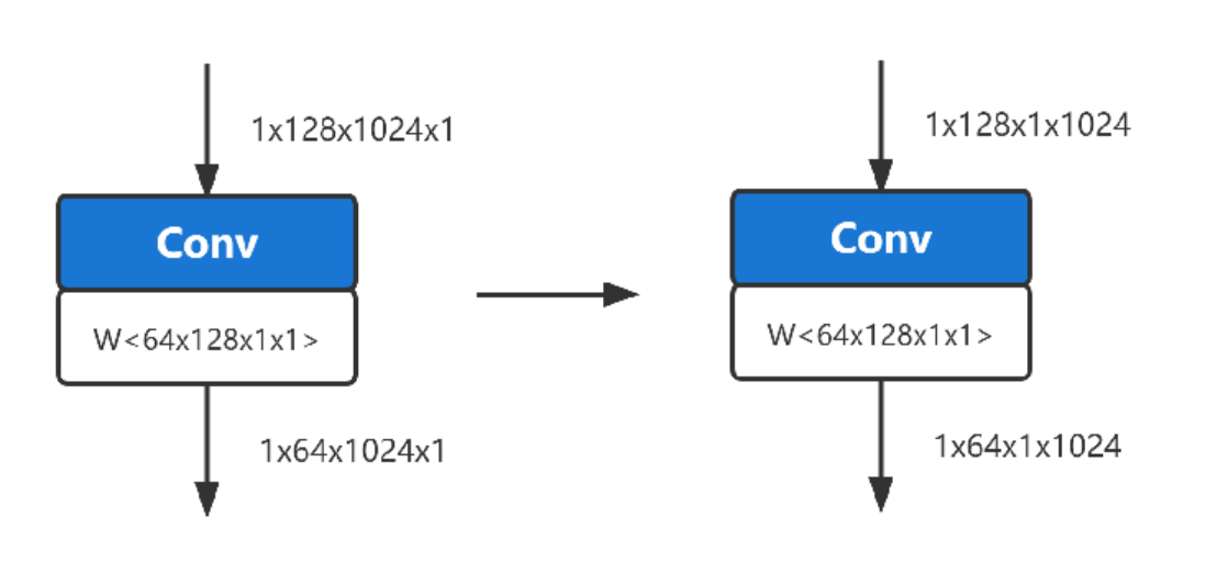
Figure 8-11 Convolution of same size comparison
8.5.2 Design of high-utilization operator
In order to improve the overall utilization of computing power in model design, it is generally necessary to avoid inefficient operators and select operator size designs that are easy to achieve higher utilization. In the following chapters, we will list some inefficient operators that can be avoided as much as possible and discuss the relationship between convolution size and utilization.
Avoid inefficient operators
Try to reduce the following three types of operators in the model
Table 8-5 Three types of inefficient operators
| Data transfer | Size transformation | Non-Relu activation function |
|---|---|---|
| Transpose | Resize | Sigmoid |
| Reshape | Tile | Tanh |
| Split | Pooling | Softplus |
| Concat | Pad | Hardswish |
Relationship between convolution size and utilization
Since the performance of convolution will be affected by both computing power and bandwidth, MAC utilization is often used to illustrate the extent of hardware computing power when evaluating performance.
The relationship between convolution size and utilization is discussed here as a performance reference aid for users to design models. The following is a rough reference based on empirical data:
Notes on the following nouns: KH (kernel height), KW (kernel width), KC (kernel channel), type_bytes (weight bit width divided by 8), Ksize (KW or KH), Kstride (stride in the KW or KH direction)
When the channel of the convolutional input and output Tensor meets the alignment requirements (see aligning table data in 8.4.1), the utilization rate is higher.
When the channel of the input Tensor is < 256, the utilization rate is relatively high. When the channel is > 512, the utilization rate will gradually decrease as the channel increases.
In terms of weight size, the utilization rate is relatively high when KH* KW * KC * type_bytes < 6K Bytes. Utilization will drop significantly when it exceeds a certain size.
The larger the ratio of Ksize / Kstride, the higher the utilization rate. For example (Ksize=3, Kstride=1 is better than Ksize=2, Kstride=1)
The utilization rate decreases when the Height * Width of the output Tensor < 16.
The larger the Channel of the output Tensor, the higher the utilization rate.
The above discussion only examines the factors that affect utilization due to independent size. The actual MAC utilization shown by convolution in the actual deployment model is the result of a combination of many factors.
8.5.3 Subgraph fusion
The RKNN software stack will match certain graph relationships into custom operators, as shown in the figure below. If they are not merged into corresponding operators, you can check whether there is no matching due to different connection relationships.
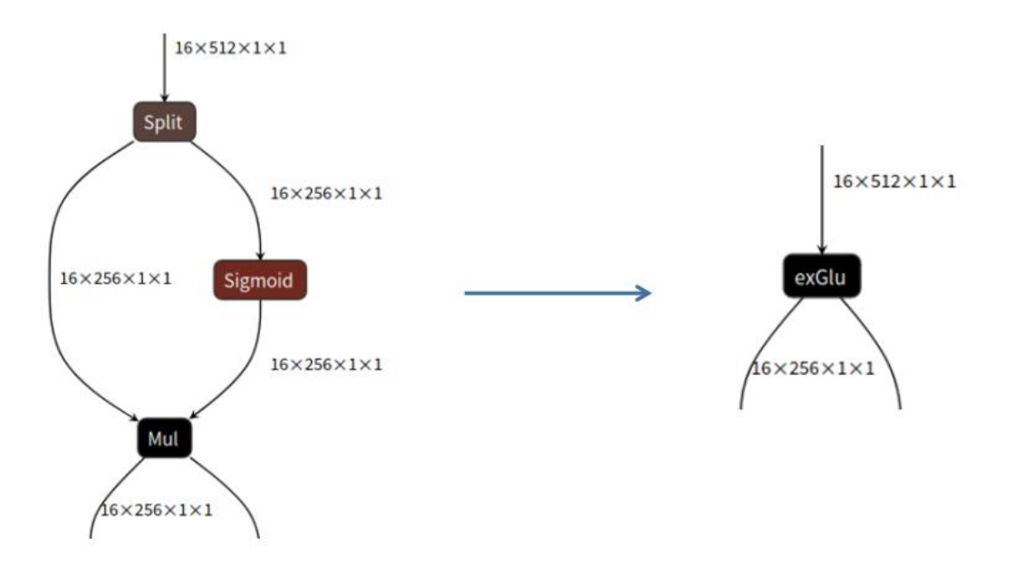
Figure 8-12 Glu subgraph fusion
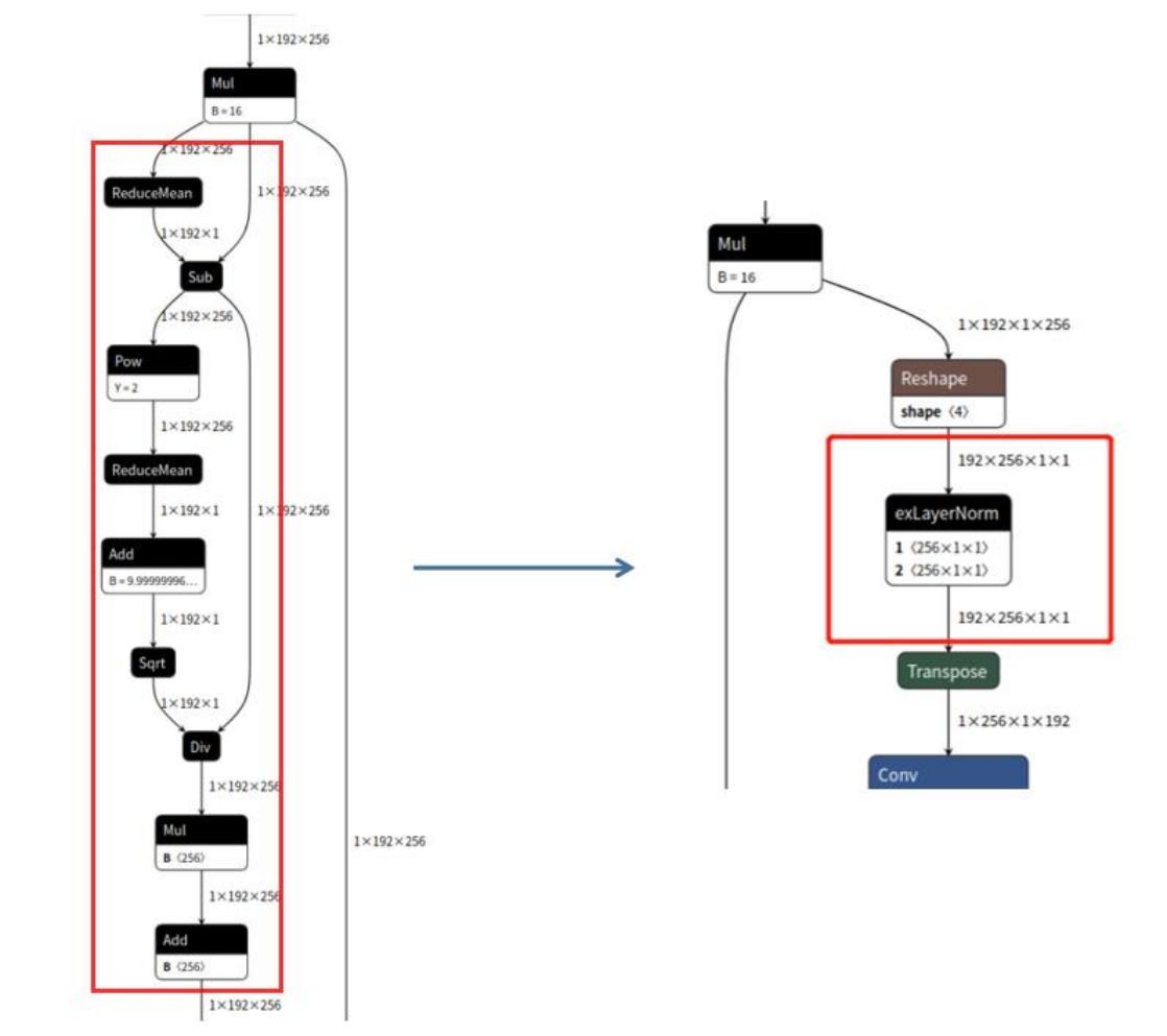
Figure 8-13 LayerNorm subgraph fusion
The supported subgraph fusion rules are:
Split + Sigmoid + Mul -> GLU
ReduceMean + Sub + Pow + ReduceMean + Add + Sqrt + Div (+ Mul + Add) -> LayerNorm
9 Memory Usage Optimization
9.1 Introduction to memory composition and analysis methods
9.1.1 Memory composition during RKNN model runtime
The RKNN model runtime memory mainly consists of four parts: weights and internal tensors, register configurations, input tensors and output tensors. Runtime memory is usually created during rknn_init.
9.1.2 Model memory analysis method
After the rknn_init() interface is called, when the user needs to view the memory allocated by the model or needs to allocate model weights externally, call the rknn_query interface and pass in RKNN_QUERY_MEM_SIZE to query the model’s weights and internal memory (excluding input and output) , the occupancy of all DMA memory and SRAM memory used for model inference (0 if SRAM is not turned on or does not have this function).
The following is the sample code:
 rknn_context ctx = 0;
 // Load RKNN Model
 int ret = rknn_init(&ctx, model_path, 0, NULL, NULL);
 if (ret < 0) {
  printf("rknn_init fail! ret=%d\n", ret);
  return -1;
 }

 // Get weight and internal mem size
 rknn_mem_size mem_size;
 ret = rknn_query(ctx, RKNN_QUERY_MEM_SIZE, &mem_size, sizeof(mem_size));
 if (ret != RKNN_SUCC) {
  printf("rknn_query fail! ret=%d\n", ret);
  return -1;
 }
 printf("total weight size: %d, total internal size: %d\n", mem_size.total_weight_size, mem_size.total_internal_size);
9.2 How to use externally allocated memory
9.2.1 Externally allocate input and output memory
According to what is mentioned in C API Zero-Copy Process, if the user uses the zero-copy API, they can allocate memory externally to the input and output tensor, and then configure it for use by the NPU. For the specific process, please refer to the flow chart in C API Zero-Copy Process. Note that to use external memory allocation, you can only use the zero-copy API. This method is mainly applicable to scenarios where users need to manually allocate memory to the NPU instead of letting the NPU allocate memory through the rknn_create_mem() interface.
External memory can be recorded using physical address and fd, and is mainly created through the following two interfaces:
rknn_create_mem_from_phys(): Create the rknn_tensor_mem structure through the physical address.
rknn_create_mem_from_fd(): Create the rknn_tensor_mem structure through the fd.
Here is an example of creating memory using mpi mmz. This example uses the rknn_create_mem_from_phys() interface to get the physical address of external memory and create a rknn tensor mem structure with physical memory information.
......

// Create input tensor memory
rknn_tensor_mem* input_mems[1];
// default input type is int8 (normalize and quantize need compute in outside)
// if set uint8, will fuse normalize and quantize to npu
input_attrs[0].type = input_type;
// default fmt is NHWC, npu only support NHWC in zero copy mode
input_attrs[0].fmt = input_layout;

input_mems[0] = rknn_create_mem_from_phys(ctx, input_phys, input_virt, input_attrs[0].size_with_stride);

......

// Create output tensor memory
rknn_tensor_mem* output_mems[io_num.n_output];
for (uint32_t i = 0; i < io_num.n_output; ++i) {
  output_mems[i] = rknn_create_mem_from_phys(ctx, output_physs[i], output_virts[i], output_attrs[i].size);
}

// Set input tensor memory
ret = rknn_set_io_mem(ctx, input_mems[0], &input_attrs[0]);
if (ret < 0) {
  printf("rknn_set_io_mem fail! ret=%d\n", ret);
  return -1;
}

// Set output tensor memory
for (uint32_t i = 0; i < io_num.n_output; ++i) {
  // set output memory and attribute
  ret = rknn_set_io_mem(ctx, output_mems[i], &output_attrs[i]);
  if (ret < 0) {
    printf("rknn_set_io_mem fail! ret=%d\n", ret);
    return -1;
  }
}
In addition to referencing the physical address of external memory, externally allocated memory can also be used by fd. The following is the sample code:
int mb_flags = RK_MMZ_ALLOC_TYPE_CMA | RK_MMZ_ALLOC_UNCACHEABLE;

// Allocate weight memory in outside
MB_BLK weight_mb;
rknn_tensor_mem* weight_mem;
ret = RK_MPI_MMZ_Alloc(&weight_mb, mem_size.total_weight_size, mb_flags);
if (ret < 0) {
  printf("RK_MPI_MMZ_Alloc failed, ret: %d\n", ret);
  return ret;
}
void* weight_virt = RK_MPI_MMZ_Handle2VirAddr(weight_mb);
if (weight_virt == NULL) {
  printf("RK_MPI_MMZ_Handle2VirAddr failed!\n");
  return -1;
}
int weight_fd = RK_MPI_MMZ_Handle2Fd(weight_mb);
if (weight_fd < 0) {
  printf("RK_MPI_MMZ_Handle2Fd failed!\n");
  return -1;
}
weight_mem = rknn_create_mem_from_fd(ctx, weight_fd, weight_virt, mem_size.total_weight_size, 0);
printf("weight mb info: virt = %p, fd = %d, size: %d\n", weight_virt, weight_fd, mem_size.total_weight_size);
9.2.2 Externally allocated model memory
In Introduction to memory composition and analysis methods, it was mentioned that model memory occupancy is divided into two parts, one part is internal memory and the other part is weight memory. If the application needs to use externally allocated model memory, it can set the model weight and the memory used by internal through the interface rknn_set_weight_mem(), rknn_set_internal_mem() interface. The following is the sample code:
// Load RKNN Model
ret = rknn_init(&ctx, model_virt, model_size, RKNN_FLAG_MEM_ALLOC_OUTSIDE, NULL);
TIME_END(rknn_init);
if (ret < 0) {
  printf("rknn_init fail! ret=%d\n", ret);
  return -1;
}

//query and inset input / output tensor
......

// Allocate weight memory in outside
MB_BLK weight_mb;
rknn_tensor_mem* weight_mem;
ret = RK_MPI_MMZ_Alloc(&weight_mb, SIZE_ALIGN_128(mem_size.total_weight_size), mb_flags);
void* weight_virt = RK_MPI_MMZ_Handle2VirAddr(weight_mb);
int weight_fd = RK_MPI_MMZ_Handle2Fd(weight_mb);

weight_mem = rknn_create_mem_from_fd(ctx, weight_fd, weight_virt, mem_size.total_weight_size, 0);

ret = rknn_set_weight_mem(ctx, weight_mem);
if (ret < 0) {
  printf("rknn_set_weight_mem fail! ret=%d\n", ret);
  return -1;
}
printf("weight mb info: virt = %p, fd = %d, size: %d\n", weight_virt, weight_fd, mem_size.total_weight_size);

// Allocate internal memory in outside
MB_BLK internal_mb;
rknn_tensor_mem* internal_mem;
ret = RK_MPI_MMZ_Alloc(&internal_mb, SIZE_ALIGN_128(mem_size.total_internal_size), mb_flags);
void* internal_virt = RK_MPI_MMZ_Handle2VirAddr(internal_mb);
int internal_fd = RK_MPI_MMZ_Handle2Fd(internal_mb);

internal_mem = rknn_create_mem_from_fd(ctx, internal_fd, internal_virt, mem_size.total_internal_size, 0);
ret = rknn_set_internal_mem(ctx, internal_mem);
if (ret < 0) {
  printf("rknn_set_internal_mem fail! ret=%d\n", ret);
  return -1;
}
printf("internal mb info: virt = %p, fd = %d, size: %d\n", internal_virt, internal_fd, mem_size.total_internal_size);
9.3 Internal Memory Reuse
The RKNN API provides a mechanism for external management of NPU memory. Through the RKNN_FLAG_MEM_ALLOC_OUTSIDE parameter, users can specify that the feature memory in the middle of the model is allocated externally. Typical application scenarios of this function are as follows:
During deployment, all NPU memory is allocated by the user, which facilitates the overall arrangement of the entire system memory.
It is used in multiple model serial running scenarios, and the intermediate feature memory is reused in different contexts, especially for devices such as RV1103/RV1106 where memory is extremely tight.
For example, there are two models in the figure below. The Internal Tensor occupancy of model 1 is larger than model 2. If model 1 and model 2 are run sequentially, the application can only allocate a memory at the address 0x00000000~0x000c4000 for model 1 and 2 to share. After the inference of Model 1, this memory can be used by Model 2 to read and write Internal Tensor data, thus saving memory.
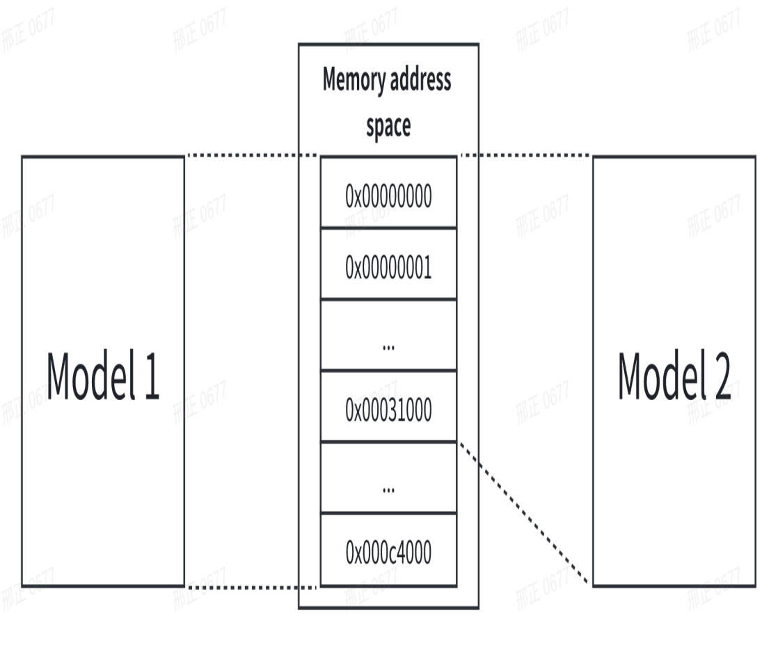
Figure 9-1 Example of two model Internal Tensors sharing the same memory address space
Assume that the path of model 1 is “model_path_a” and the path of model 2 is “model_path_b”. The sample code is as follows:
rknn_init(&ctx_a, model_path_a, 0, RKNN_FLAG_MEM_ALLOC_OUTSIDE, NULL);
rknn_query(ctx_a, RKNN_QUERY_MEM_SIZE, &mem_size_a, sizeof(mem_size_a));

rknn_init(&ctx_b, model_path_b, 0, RKNN_FLAG_MEM_ALLOC_OUTSIDE, NULL);
rknn_query(ctx_b, RKNN_QUERY_MEM_SIZE, &mem_size_b, sizeof(mem_size_b));

// Get the largest internal size of the two models
max_internal_size = MAX(mem_size_a.total_internal_size, mem_size_b.total_internal_size);
internal_mem_max = rknn_create_mem(ctx_a, max_internal_size);
// Set a model internal memory
internal_mem_a = rknn_create_mem_from_fd(ctx_a, internal_mem_max->fd,
internal_mem_max->virt_addr, mem_size_a.total_internal_size, 0);
rknn_set_internal_mem(ctx_a, internal_mem_a);
// Set b model internal memory
internal_mem_b = rknn_create_mem_from_fd(ctx_b, internal_mem_max->fd,
internal_mem_max->virt_addr, mem_size_b.total_internal_size, 0);
rknn_set_internal_mem(ctx_b, internal_mem_b);
9.4 Multi-threaded Reuse RKNN Context
In a multi-threaded scenario, a model may be executed by multiple threads at the same time. If each thread initializes a context separately, the memory consumption will be very large. Therefore, the application can consider sharing a context to avoid repeated memory allocation of RKNN context and reduce runtime memory usage.
The RKNN API provides an interface for reusing contexts. The interface is defined as follows:
int rknn_dup_context(rknn_context* context_in,rknn_context* context_out)
The context_in is the initialized context, and context_out is the context that reuses context_in.
As shown in the figure below, the model structure of the two contexts is the same, so the contexts can be reused.
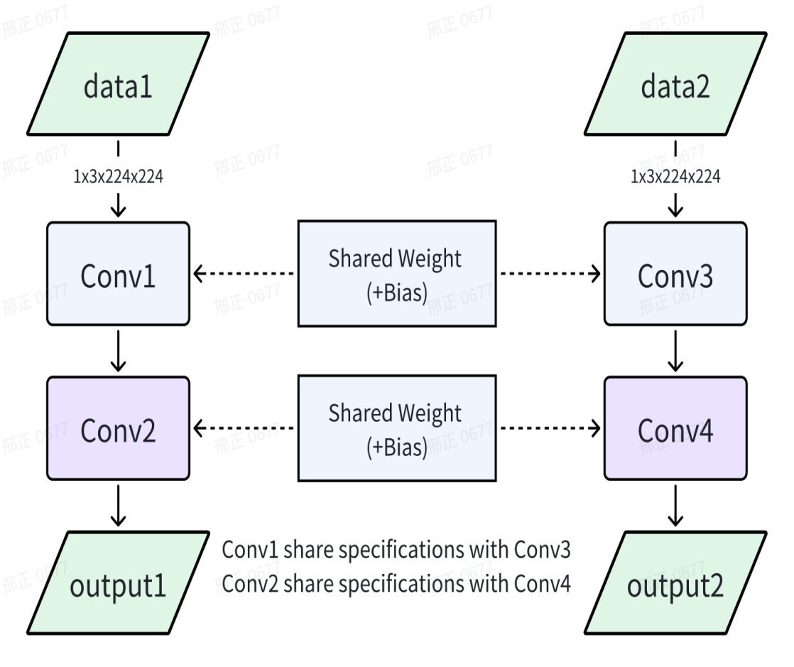
Figure 9-2 Example of two identical model reuse contexts
9.5 Multiple resolution models share the same weights
When multiple models with different resolutions have the same weight, they can share the same weight to reduce memory usage. When the version of RKNPU SDK is equal or below 1.5.0, this function can realize dynamic switching between different resolution models with a small memory footprint. After version 1.5.0, this function is replaced by the dynamic shape function.
As shown in the figure below, the weights of model A and model B are exactly the same.
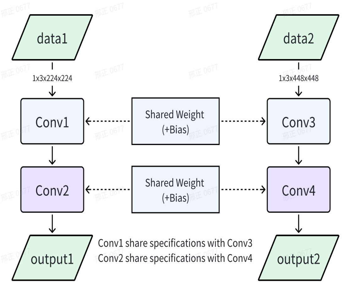
Figure 9-3 Example of two models with different resolutions sharing weights
The application can follow the following steps to achieve multi-resolution models sharing the same weights:
1. When converting the RKNN model, one of the models is set as the master model, the rknn.config interface sets the parameter remove_weight=False, and the other model is set as the slave model, and the parameter remove_weight=True is set. The master RKNN model contains weights, and the slave RKNN model does not contain convolutional class weights.
2. When deploying, initialize the master RKNN model first, and then initialize the slave RKNN model. When initializing the slave model, use the RKNN_FLAG_SHARE_WEIGHT_MEM flag and add the rknn_init_extend parameter. This parameter value is the context of the master model. Assume that the main model path is “model_A” and the slave model path is “model_B”. The sample code is as follows:
rknn_context context_A;
rknn_context context_B;
ret = rknn_init(&context_A,model_A,0,0,NULL);
...
rknn_init_extend extend;
extend.ctx = context_A;
ret = rknn_init(&context_B,model_B,0,RKNN_FLAG_SHARE_WEIGHT_MEM,&extend);
10 Trouble Shooting
10.1 NPU SDK environment problem
Version compatibility
NPU kernel driver & Runtime
It is recommended to upgrade the NPU kernel driver to version 0.9.2 or later. When encountering problems, try to resolve problem by updating latest NPU kernel driver version.
RKNN model(determined by RKNN-Toolkit2) & Runtime:
Table 10-1 Correspondence between RKNN model and Runtime version
| RKNN model version | Runtime version |
|---|---|
| 1.2.0 | >=1.2.0 and <=1.5.0 |
| 1.3.0 | >=1.3.0 and <=1.5.0 |
| 1.4.0 | >=1.4.0 and <=1.5.0 |
| 1.5.0 | 1.5.0 |
| 1.5.2 | >=1.5.2 |
| 1.6.0 | >=1.5.2 |
| 2.0.0 | >=2.0.0 |
| 2.1.0 | >=2.1.0 |
How to update the NPU kernel driver
It is recommended to upgrade the complete firmware to upgrade the NPU driver. The corresponding firmware needs to be provided by the board manufacturer.
Using NPU in Docker
Map NPU resources to the specific path when starting the Docker container. The reference commands are as follows:
docker run -t -i --privileged -v /dev/dri/renderD129:/dev/dri/renderD129 -v /proc/device-tree/compatible:/proc/device-tree/compatible -v /usr/lib/librknnrt.so:/usr/lib/librknnrt.so ai_application:v1.0.0 /bin/bash
Parameter explanation:
/dev/dri/renderD129 is RK3588’s NPU device node. Runtime relies on this node to enable NPU.
/proc/device-tree/compatible records the SOC model. Components such as RKNN-Toolkit Lite2 rely on this file to obtain the current SOC information.
/usr/lib/librknnrt.so is the Runtime file. RKNN-Toolkit Lite2 and RKNPU2 C API relies on this file to use NPU resources.
ai_application:v1.0.0 means <Docker image name>:<version>.
10.2 RKNN-Toolkit2 installation issue
Too strict dependencies hinder the installation of RKNN-Toolkit2
All dependent libraries have been installed, but the versions and requirements of some libraries do not match, you can try adding the –no-deps parameter after the installation command to cancel the environment check when installing the Python wheel package:
pip install rknn-toolkit2*.whl --no-deps
PyTorch dependency
The recommended PyTorch versions are version 1.6.0, 1.9.0, 1.10 or 1.13.1.
The PyTorch model loading function depends on PyTorch lib. PyTorch’s models are divided into floating-point models and quantized models (including QAT and PTQ quantized models).
For models exported by PyTorch 1.6.0, it is recommended to downgrade the PyTorch version that RKNN-Toolkit2 depends on to avoid loading model failures.
For quantized models (QAT, PTQ), we recommend using PyTorch 1.10~1.13.1 to export the model and upgrade the PyTorch version that RKNN-Toolkit2 depends on to 1.10~1.13.1.
In summary, the PyTorch version used for exporting models is recommended to be as consistent as possible with the PyTorch version that RKNN-Toolkit2 depends on.
TensorFlow dependency
The recommended TensorFlow versions are version 2.6.2, 2.8.0.
The TensorFlow model loading function of RKNN-Toolkit2 relies on TensorFlow lib. Due to the general compatibility between TensorFlow versions, other versions may cause RKNN-Toolkit2 loading model errors. Therefore, the Tensorflow version used for exporting models is recommended to be as consistent as possible with the Tensorflow version that RKNN-Toolkit2 depends on.
Problems caused by the TensorFlow version are usually reflected in the rknn.load_tensorflow() stage, and the error message will point to the dependent TensorFlow lib path.
RKNN-Toolkit2 installation package naming rules
Taking the release version 1.5.2 as an example, the RKNN-Toolkit2 wheel package naming rules are as follows:
rknn_toolkit2-1.5.2+b642f30c-cp38-cp38-linux_x86_64.whl
rknn_toolkit2: tool name.
1.5.2: version.
b642f30c: commit id.
cp<xx>-cp<xx>: Applicable Python version, for example cp38-cp38 means the applicable Python version is 3.8.
linux_x86_64: System type and CPU architecture.
Either a mismatched system type, CPU architecture, or Python version will cause the RKNN-Toolkit2 installation failure.
RKNN-Toolkit2 ARM Linux version available?
No ARM Linux version. If you need to use the Python interface for inference on ARM Linux, you can install RKNN-Toolkit-lite2, which supports running inference using Python on ARM Linux. bfloat16 lib installation failure
One error occurred during the installation of bfloat16 lib as follows:
The original screenshot is clipped; only visible text is transcribed. Missing portions are not reconstructed.
bfloat16.cc:2013:57: note: expected a type, got ‘bfloat16’
bfloat16.cc:2013:57: error: type/value mismatch at argument 2 in templa
e, class Functor> struct greenwaves::{anonymous}::UnaryUFunc’
bfloat16.cc:2013:57: note: expected a type, got ‘bfloat16’
bfloat16.cc:2015:67: error: ‘>>’ should be ‘> >’ within a nested templa
RegisterUFunc<BinaryUFunc<bfloat16, bfloat16, ufuncs::NextAfter>>(
                                                               ^
bfloat16.cc:2015:58: error: type/value mismatch at argument 1 in templa
e, class Functor> struct greenwaves::{anonymous}::BinaryUFunc’
RegisterUFunc<BinaryUFunc<bfloat16, bfloat16, ufuncs::NextAfter>>(
Figure 10-1 bfloat16 dependent library installation failure log
Change the pip source to Alibaba source, or update RKNN-Toolkit2 to 1.5.0 and later versions (1.5.0 and later versions have removed the dependency on the bfloat16 library)
10.3 Model conversion parameters description
This chapter mainly covers the usage instructions of commonly used parameters in the model conversion stage.
Parameters determined by model
During model conversion, the rknn.config() and rknn.build() interfaces will affect the model conversion results. rknn.load_onnx, rknn.load_tensorflow() specifies the input and output nodes, which will affect the model conversion results. The size of the inputs specified by rknn.load_pytorch() and rknn.load_tensorflow() will affect the model conversion results.
Referring to the following basic steps for model conversion:
1. Prepare quantitative data and provide the dataset.txt file.
2. Determine the NPU platform, such as RK3566, RV1106, etc., and fill in the target_platform parameter in the rknn.config() interface.
3. When the input is a 3-channel image and the quantified data is in image format (such as jpg, png format), you need to confirm whether the input of the model is RGB or BGR to determine the value of the quant_img_RGB2BGR parameter in the rknn.config() interface.
4. Confirm the normalization parameters during model training to determine the values of the mean_values and std_values parameters in the rknn.config interface.
5. Confirm the input size of the model and fill in the corresponding parameters of the load interface, such as the input_size_list parameter in the rknn.load_pytorch() interface.
6. Confirm that the model requires quantized bits to determine the value of the quantized_dtype parameter in the rknn.config() interface. This step can be ignored if the model needsn’t be quantized or loading an already quantized model.
7. Confirm the quantization algorithm used in model quantization to determine the value of the quantized_algorithm parameter in the rknn.config() interface. This step can be ignored if the model needsn’t be quantized or loading an already quantized model.
8. Confirm whether the model needs quantization to determine the value of the do_quantization parameter in the rknn.build() interface. When enabling quantization, dataset parameter in the rknn.build() interface is required to specify the quantization data. Cross-platform compatibility of RKNN models
For the platform parameters set by target_platform in rknn.config(), the compatibility relationship is as follows:
RK3566’s RKNN model can be used on RK3568.
RK3588’s RKNN model can be used on RK3588s.
RV1106’s RKNN model can be used on RV1103.
Format and requirements of quantization data
There are two formats for quantization data. One is the image(jpg, png), RKNN-Toolkit2 will call the OpenCV interface to read; the other is npy format, RKNN-Toolkit2 will call the numpy to read.
For models with non-RGB/BGR image input, it is recommended to use numpy’s npy format to provide quantization data.
Filling format of dataset.txt file for multi-input model
Model quantization requires the dataset.txt file to specify the path of quantization data. The rule is that one line serves as a set of inputs. When the model has multiple inputs, multiple inputs are written on the same line and separated by spaces.
For example, a single-input model with two sets of quantization data:
sampleA.npy
sampleB.npy
For example, a three-input model with two sets of quantization data:
sampleA_in0.npy sampleA_in1.npy sampleA_in2.npy
sampleB_in0.npy sampleB_in1.npy sampleB_in2.npy
Confirm the quant_img_RGB2BGR parameter of rknn.config()
When using images (jpg, png) as quantization data, the quant_img_RGB2BGR parameter should be counted in consideration.
When the model uses RGB images for training, set the quant_img_RGB2BGR parameter as False or ignore setting. Then use RGB images as the input for both Python API and RKNPU2 CAPI inference interface.
When the model uses BGR images for training, set the quant_img_RGB2BGR parameter as True. Then use BGR images as the input for both Python API and RKNPU2 CAPI inference interface. (quant_img_RGB2BGR will only affect reading images in the quantization step).
If the quantization data is saved as numpy’s npy format, it is recommended not to use the quant_img_RGB2BGR parameter to avoid confusion.
Calculation order of mean, std, and quant_img_RGB2BGR in rknn.config()
The quant_img_RGB2BGR parameter only affects reading images in the quantization step. It no longer affects other steps.
Therefore, for the inference interface of RKNN-Toolkit2 Python API and RKNPU2 C API, the input data first performed Mean subtraction, followed by std division, and then fed to the RKNN model.
Setting mean_valuesandstd_values in rknn.config() inference for model with non-3-channel input or multi-input.
The setting formats of mean_values and std_values are consistent. Take mean_values as an example.
Assuming that the input has N channels, the value of mean_values is [[channel_1, channel_2, channel_3, channel_4, …, channel_n]].
When there are multiple inputs, the value of mean_values is [[channel_1, channel_2, channel_3, channel_4, …, channel_n], [channel_1, channel_2, channel_3, channel_4, …, channel_n]].
Quantization algorithm and selection of the number of quantized pictures
RKNN-Toolkit2’s quantization algorithm (quantized_algorithm of rknn.config()) provides three algorithms for quantization parameters correction, namely normal, mmse, and kl_divergence. The normal is used by default.
The normal is a basic quantization algorithm.
The mmse will iterate the calculation results of the intermediate layer and clip the weight values within a certain range to obtain higher inference accuracy. Using mmse may not certainly improve the quantization accuracy, but compared with the normal method, quantization will occupy more memory and cast more time.
The kl_divergence will take more time than normal, but much less time than mmse. In some scenarios (when the feature distribution is uneven), better improvement results can be obtained.
It is recommended to use the normal first. If the quantization accuracy is not good, try to use the mmse or kl_divergence.
For normal or kl_divergence, 20-200 sets of data are recommended. For mmse, 20-50 sets of data are recommended.
Difference between input and output during inference, compared with Quantized and non-quantized models
When calling the general RKNPU2 C API (meaning calling the C API without using pass_through or zero_copy), the data type of the input data (such as uint8 data, float data) has nothing to do with whether the model is quantized or not. The output data can be automatically processed into float32 format, or keeping format as the model defined. There will be some differences when using the Python inference interface. The specific relationship is as follows:
Table 10-2 Differences between Python inference interface and general C API interface
| After model quantization |
Python inference interface(rknn.inference()) |
C API inference interface(rknn.run()) (Non pass_through、zero_copy) |
|---|---|---|
| Input type restrictions |
No restrictions. The input of rknn.inference() is a list of numpy arrays with a data type attribute. The input will be automatically converted into the data type required by the RKNN model. |
No restrictions. The rknn_tensor_type parameter of rknn_inputs can specify RKNN_TENSOR_FLOAT32, RKNN_TENSOR_FLOAT16, RKNN_TENSOR_INT8, RKNN_TENSOR_UIN8, RKNN_TENSOR_INT16 according to the actual input. After specifying, the input will be automatically converted into the data type required by the RKNN model. |
| Has output data type changed? |
Not changed. Regardless of whether quantized or not, Python’s rknn.inference() interface always returns float type output. No other data type can be specified. |
Changed. For RKNPU2 C API, rknn outputs attr can be set want_float=1 to get an float output. After quantization, want_float=0 can be set to get an output with the data type as model defined. For example, if quantized as i8, int8 data outputs. |
| Has input format changed (NCHW, NHWC)? |
Not changed. Regardless of whether the model is quantized or not, the data_format parameter of the rknn.inference() interface can be set to nchw or nhwc as needed. |
Changed. Regardless of whether the model is quantized or not, the rknn_tensor_format parameter of the rknn inputs’ structure can be set to NCHW or NHWC as needed |
Is there an online precompiled mode
RKNN-Toolkit2 only supports exporting offline precompiled models and does not support exporting online precompiled models (which is supported by RKNN-Toolkit1), so there is no mode selection between offline precompilation and online precompilation.
Can the RKNN model converted from RKNN-Toolkit be used on the RK3566 platform
It can’t.
The RKNN model converted from RKNN-Toolkit is suitable for RK1806 / RK1808 / RK3399Pro / RV1109 / RV1126 platforms; the RK3566 platform requires the RKNN model converted from RKNN-Toolkit2. The RKNN model converted from RKNN-Toolkit2 is suitable for platforms such as RK2118/ RV1103B/ RV1103 / RV1106B / RV1106 / RV1126B / RK3562 / RK3566 / RK3568 / RK3576/ RK3588.
For instructions on using the RKNN-Toolkit, please refer to the following project:https://github.com/airockc hip/rknn-toolkit
For instructions on using the RKNN-Toolkit2, please refer to the following project:https://github.com/airock chip/rknn-toolkit2
10.4 Deep-learning framework FAQs
10.4.1 Deep learning frameworks and corresponding versions supported by RKNN-Toolkit2
Please refer to Chapter 3.1.
10.4.2 OP support list for each framework
RKNN-Toolkit2 has different support levels for different frameworks. For detailed information, please refer to the RKNNToolkit2_OP_Support document in the following link:
https://github.com/airockchip/rknn-toolkit2/blob/master/doc/
10.4.3 FAQs about ONNX model conversion
“Error parsing message” appears when loading the model
For example, converting the examples/onnx/resnet50v2 model fails and the prompt is as follows:
E load_onnx: Catch exception when loading onnx model: /rknn_resnet_demo/resnet50v2.onnx!

E lod_onnx: Traceback (most recent call last):

E load_onnx: File "rknn/api/rknn_base.py", line 1094, in rknn.api.rknn_base.RKNNBase.load_onnx

E load_onnx: File "/usr/local/lib/python3.6/dist-packages/onnx/__init__.py", line 115, in load_model

……

E load_onnx: google.protobuf.message.DecoderError: Error parsing message
The reason may be that the resnet50v2.onnx model is damaged (if the entire model is not downloaded). Re- download the model and ensure that its MD5 value is correct, such as:
22ed6e6a8fb9192f0980acca0c941414 resnet50v2.onnx
Is dynamic input shape supported?
For example, the input dimension of ONNX is [-1, 3, -1, -1], which means that the batch, height and width dimensions are not fixed. RKNN-Toolkit2 before 1.5.2 version does not support dynamic input shape.
Versions 1.5.2 and later support dynamic input shapes through the dynamic_input parameter of rknn.config(), see Chapter 5.4 for details.
An error occurs when customizing the output node
For example, calling rknn.load_onnx() with setting outputs parameter and the error occurs as follows.
E load_onnx: the '378' in outputs=['378', '439', '500'] is invalied!
The log prompts that output node 378 is invalid. It means that the outputs parameter needs to be set to the correct output node name.
10.4.4 FAQs about Pytorch model conversion
An error occurs when loading a Pytorch model: torch._C does not have the _jit_pass_inline attribute
The error log is as follows:
'torch._C' has no attribute '_jit_pass_inline'
Please upgrade PyTorch to version 1.6.0 or later.
Saving format of Pytorch models
Currently, only models exported by torch.jit.trace() are supported. The torch.save() interface only saves the weight parameter dictionary, which lacks network structure information and cannot be normally imported and converted into an RKNN model.
PytorchStreamReader failed during the conversion
The error log is as follows:
E Catch exception when loading pytorch model: ./mobilenet0.25_Final.pth!

E Traceback (most recent call last):

……

E cpp_module = torch._C.import_ir_module(cu, f, map_location, extra_files)

E RuntimeError: [enforce fail at inline container.cc:137]. PytorchStreamReader failed reading zip archive: faild
finding central directory frame #0 ……
The reason is that the PyTorch model does not have network structure information.
Usually .pth file only contains weights but not network structure information. To export a model with the network structure, initialize the corresponding network structure and then use net.load_state_dict() to load the .pth weight file. Next, use torch.jit.trace() interface to solidify the network structure and weight. Finally, use torch.jit.save() to save the traced model in .pt format, which can be used for the rknn.load_pytorch() interface to convert it into an RKNN model. KeyError encountered during conversion
The error log is as follows:
E Traceback (most recent call last):

……

E KeyError: 'aten::softmax'
When an error message in the form of KeyError: ‘aten::xxx’ appears, it means that the current version of the operator does not support it. RKNN-Toolkit2 will fix such bugs every time it is upgraded. Please use the latest version of RKNN-Toolkit2 to solve it.
“Syntax error in input! LexToken(xxx)” error encountered during conversion
The error log is as follows:
WARNING: Token 'COMMENT' defined, but not used

WARNING: There is 1 unused token

!!!!! Illegal character '"'

Syntax error in input! LexToken(NAMED_IDENTIFIER, 'fc', 1, 27)

!!!!! Illegal character '"'
There are many reasons for this error. Please troubleshoot in the following order:
1)The torch.nn.module is not inherited to create the network. Please inherit the torch.nn.module class type to create the network, and then use torch.jit.trace() to generate the pt file.
2)To update RKNN-Toolkit2 1.4.0 or later version, torch recommends version 1.6.0, 1.9.0, 1.10.0 or 1.13.1.
10.4.5 FAQs about Tensorflow model conversion
Tensorflow1.x model error
Loading tensorflow1.x model with rknn.load_tensorflow() interface, an error message appears:
E load_tensorflow: Catch exception when loading tensorflow model: ./yolov3_mobilenetv2.pb!

E load_tensorflow: Traceback (most recent call last):

……

E load_tensorflow: tensorflow.python.framework.errors_impl.InvalidArgumentError: Node
'MobilenetV2/expanded_conv/depthwise/BatchNorm/cond/Switch_1' expects to be colocated with unknown node
'MobilenetV2/expanded_conv/depthwise/BatchNorm/moving_mean'

E load_tensorflow: During handling of the above exception, another exception occurred:

E load_tensorflow: Traceback (most recent call last):

E load_tensorflow: File "rknn/api/rknn_base.py", line 990, in rknn.api.rknn_base.RKNNBase.load_tensorflow

……

E load_tensorflow: return func(*args, **kwargs)

E load_tensorflow: File "/usr/local/lib/python3.6/dist-packages/tensorflow/python/framework/importer.py", line
431, in import_graph_def

E load_tensorflow: raise ValueError(str(e))

E load_tensorflow: ValueError: Node 'MobilenetV2/expanded_conv/depthwise/BatchNorm/cond/Switch_1' expects
to be colocated with unknown node 'MobilenetV2/expanded_conv/depthwise/BatchNorm/moving_mean'
Suggestion:
If TensorFlow 1.x is currently installed, please update to TensorFlow 2.x.
Update RKNN-Toolkit2/RKNPU2 to the latest version.
TransformGraph error
The error log is as follows:
Traceback (most recent call last):

File "test.py", line 80, in <module>

input_size_list=[[1, 368, 368, 3]])

File "/usr/local/lib/python3.6/site-packages/rknn/api/rknn.py", line 68, in load_tensorflow

input_size_list=input_size_list, outputs=outputs)

File "rknn/api/rknn_base.py", line 940, in rknn.api.rknn_base.RKNNBase.load_tensorflow
File "/usr/local/lib/python3.6/dist-packages/tensorflow/tools/graph_transforms/__init__", line 51, in
TransformGraph.transforms_string, status)

File "/usr/local/lib/python3.6/dist-packages/tensorflow/python/framework/errors_impl.py". ;ome 548, in __exit__

C_api.TF_GetCode(self.status.status)

Tensorflow.python.framework.error_impl.InvalidArgumentError: Beta input to batch norm has bad shape: [24]
Reason:
1)RKNN-Toolkit2 calls TensorFlow’s native TransformGraph function for the model optimization but it fails.
2)One probable reason is that the TensorFlow version used for exporting the model is no longer compatible with the currently installed version.
Suggestion:
Use TensorFlow version 1.14.0 to export the model, or find the same type of model in other deep-learning frameworks. “Shape must be rank 4 but is rank 0” error
When loading the pb model with the command as follows:
  rknn.load_tensorflow(tf_pb='./model.pb',

  inputs=["X","Y"],

  outputs=['generator/xs'],

  input_size_list=1, INPUT_SIZE, INPUT_SIZE, 3)
Error occurs:
  E load_tensorflow: Catch exception when loading tensorflow model: ./model.pb!

  E load_tensorflow: Traceback (most recent call last):

  E load_tensorflow: File "/usr/local/lib/python3.6/dist-packages/tensorflow/python/framework/importer.py", line
427, in import_graph_def

  E load_tensorflow: graph._c_graph, serialized, options) # pylint: disable=protected-access

  E load_tensorflow: tensorflow.python.framework.errors_impl.InvalidArgumentError: Shape must be rank 4 but is
rank 0 for 'generator/conv2d_3/Conv2D' (op: 'Conv2D') with input shapes: [], [7,7,3,32].
The reason may be that the model is a multi-input model and the input_size_list of rknn.load_tensorflow() is not filled in according to the specifications. Please refer to the following usage in examples/functions/multi_input_test:
  rknn.load_tensorflow(tf_pb='./conv_128.pb',

  inputs=['input1', 'input2', 'input3', 'input4'],

  outputs=['output'],

  input_size_list=[[1, 128, 128, 3], [1, 128, 128, 3],

  [1, 128, 128, 3], [1, 128, 128, 1]])
Troubleshooting when loading model errors
First confirm whether the original deep-learning framework can load the model and invoke it correctly.
Secondly, please upgrade RKNN-Toolkit2 to the latest version. If the model has layers (or OPs) that RKNN- Toolkit2 does not support, the debug log should prompt it. If needed, call RKNN(verbose=True) to enable more conversion logs.
If it still cannot be solved, please provide the RKNN-Toolkit2 version and the detailed error log to the Rockchip NPU development team.
10.5 Model Quantification Issues
Quantization effect on model size
There are two situations. When the imported model is a quantized model, do_quantization=False of the rknn.build() interface will use the quantization parameters in the model. When the imported model is a floating-point model, do_quantization=False will not perform quantization operations, but will convert the weights from float32 to float16, with almost no accuracy loss. Both cases reduce the size of the model size, thereby making the entire model take up less space.
When quantizing the model, does the image need to be consistent with the size of the model input?
Unnecessary.
RKNN-Toolkit2 will automatically resize these images. However, the resize operation may also change the image information and have a certain impact on the quantization accuracy, so it is best to use images matching the input size.
If the correction data is in a non-image format, such as npy format, it needs to be consistent with the shape input by the model.
Whether the quantization correction data needs to be modified according to the rknn_batch_size parameter
Unnecessary.
The rknn_batch_size parameter of rknn.build() will only modify the batch dimension of the finally exported RKNN model (from 1 to rknn_batch_size), and will not affect the process of the quantization stage. Therefore, the quantization correction data should be prepared like a non-batch model.
While quantizing model, the conversion program is stuck or killed after a period of time
During the model quantization process, RKNN-Toolkit2 will allocate partitioned system memory, which may cause the program to be killed or stuck.
Solution: Increase computer memory or increase virtual memory (swap partition).
10.6 Model conversion issues
Common conversion bugs
If encounter a conversion error similar to the following, it is likely due to a bug in the current version. You can try to update RKNN-Toolkit2 to the latest version.
infer_shapes similar error
  (op_type:Mul, name:Where_2466_mul): Inferred elem type differs from existing elem type: (FLOAT) vs
(INT64)

  E build: Catch exception when building RKNN model!

  E build: Traceback (most recent call last):

  E build: File "rknn/api/rknn_base.py", line 1555, in rknn.api.rknn_base.RKNNBase.build

  E build: File "rknn/api/graph_optimizer.py", line 5409, in rknn.api.graph_optimizer.GraphOptimizer.run

  E build: File "rknn/api/graph_optimizer.py", line 5123, in
rknn.api.graph_optimizer.GraphOptimizer._fuse_ops

  E build: File "rknn/api/ir_graph.py", line 180, in rknn.api.ir_graph.IRGraph.rebuild

  E build: File "rknn/api/ir_graph.py", line 140, in rknn.api.ir_graph.IRGraph._clean_model

  E build: File "rknn/api/ir_graph.py", line 56, in rknn.api.ir_graph.IRGraph.infer_shapes

  E build: File "/home/anaconda3/envs/rk2/lib/python3.6/site-packages/onnx/shape_inference.py", line 35, in
infer_shapes

  E build: inferred_model_str = C.infer_shapes(model_str, check_type)

  E build: RuntimeError: Inferred elem type differs from existing elem type: (FLOAT) vs (INT64)
or:
  E build: Traceback (most recent call last):

  E build: File "rknn/api/rknn_base.py", line 1643, in rknn.api.rknn_base.RKNNBase.build

  E build: File "rknn/api/graph_optimizer.py", line 6256, in
rknn.api.graph_optimizer.GraphOptimizer.fuse_ops

  E build: File "rknn/api/ir_graph.py", line 285, in rknn.api.ir_graph.IRGraph.rebuild

  E build: File "rknn/api/ir_graph.py", line 149, in rknn.api.ir_graph.IRGraph._clean_model

  E build: File "rknn/api/ir_graph.py", line 62, in rknn.api.ir_graph.IRGraph.infer_shapes

  E build: File "/usr/local/lib/python3.6/dist-packages/onnx/shape_inference.py", line 35, in infer_shapes

  E build: inferred_model_str = C.infer_shapes(model_str, check_type)
  E build: RuntimeError: Inferred shape and existing shape differ in rank: (0) vs (3)
or:
  (op_type:ReduceMax, name:ReduceMax_18): Interred shape and existing shape differ in rank: (3) vs (0)

  E build: Catch exception when building RKNN model!

  E build: Traceback (most recent call last):

  ……

  E build: RuntimeError: Interred shape and existing shape differ in rank: (3) vs (0)
_p_fuse_two_mul similar error
  E build: Catch exception when building RKNN model!

  E build: Traceback (most recent call last):

  E build: File "rknn/api/rknn_base.py", line 1643, in rknn.api.rknn_base.RKNNBase.build

  E build: File "rknn/api/graph_optimizer.py", line 6197, in
rknn.api.graph_optimizer.GraphOptimizer.fuse_ops

  E build: File "rknn/api/graph_optimizer.py", line 204, in rknn.api.graph_optimizer._p_fuse_two_mul

  E build: ValueError: non-broadcastable output operand with shape () doesn't match the broadcast shape
(3,2)
“Segmentation fault” similar error
Such as picodet model conversion error:
 I _fold_constant remove nodes = ['Shape_0', 'Gather_4', 'Shape_1', 'Gather_6', 'Unsqueeze_0',
'Concat_8', 'Cast_3']

Segmentation fault (Core dumped)
_p_fuse_mul_into_conv similar error
E build: Catch exception when building RKNN model:

……
E build: ValueError: non broadcastable output operand whith shape (1,258,1,256) doesn`t match the
broadcast shape (80256,258,1,256)
How to judge whether the OP is supported in RKNN
Convert the model directly. If it is not supported, there will be relevant prompts.
You can also refer to the following two operator support documents:
The doc/RKNNToolKit2_OP_Support-x.x.x.md document of the RKNN-Toolkit2 release package, which is a rough support list for each framework.
The doc/RKNN_Compiler_Support_Operator_List_vx.x.x.pdf document of the RKNPU2 release package contains detailed RKNN operator specifications. It prompts that the ‘expand’ is not supported
Suggest:
1. The new version already supports ‘Expand’ of CPU, you can try to update RKNN-Toolkit2 / RKNPU2 to the latest version.
2. Modify the model and use ‘Repeat’ instead of ‘Expand’.
Tips “Meet unsupported dims in reducesum”
Model conversion appears “Meet unsupported dims in reducesum, dims: 6”, as follows:
D RKNN: [14:54:19.434] >>>>>> start: N4rknn17RKNNInitCastConstE

D RKNN: [14:54:19.434] <<<<<<<< end: N4rknn17RKNNInitCastConstE

D RKNN: [14:54:19.434] >>>>>> start: N4rknn20RKNNMultiSurfacePassE

D RKNN: [14:54:19.434] <<<<<<<< end: N4rknn20RKNNMultiSurfacePassE

D RKNN: [14:54:19.434] >>>>>> start: N4rknn14RKNNTilingPassE

D RKNN: [14:54:19.434] <<<<<<<< end: N4rknn14RKNNTilingPassE

D RKNN: [14:54:19.434] >>>>>> start: N4rknn23RKNNProfileAnalysisPassE

D RKNN: [14:54:19.434] <<<<<<<< end: N4rknn23RKNNProfileAnalysisPassE

D RKNN: [14:54:19.434] >>>>>> start: OpEmit

E RKNN: [14:54:19.438] Meet unsupported dims in reducesum, dims: 6

Aborted (core dumped)
At present, RKNN does not support 6-dimensional OP. In most cases, it only supports 4-dimensional. Other dimensions will have some limitations.
Conversion error by NonMaxSuppression
Post-processing Ops such as NonMaxSuppression, RKNN currently do not support.
The post-processing subgraph part of the graph can be removed, such as:
rknn.load_onnx(model='picodet_xxx.onnx', outputs=['concat_4.tmp_0', 'tmp_16'])
The removed subgraphs are processed separately on the CPU side.
“invalid expand shape” similar error
For example, the following error occurs when rvm_mobilenetv3_fp32.onnx is converted:
[E:onnxruntime:, sequential_executor.cc:333 Execute] Non-zero status code returned while running Expand node.
Name:'Expand_294' Status Message: invalid expand shape

E build: Catch exception when building RKNN model!
E build: Traceback (most recent call last):

E build: File "rknn/api/rknn_base.py", line 1638, in rknn.api.rknn_base.RKNNBase.build

E build: File "rknn/api/graph_optimizer.py", line 5529, in rknn.api.graph_optimizer.GraphOptimizer.fold_constant

E build: File "rknn/api/session.py", line 69, in rknn.api.session.Session.run

E build: File "/home/cx/work/tools/Anaconda3/envs/rknn/lib/python3.8/site-packages/onnxruntime/capi/onnxruntime_inference_collection.py", line 124, in run

E build: return self._sess.run(output_names, input_feed, run_options)

E build: onnxruntime.capi.onnxruntime_pybind11_state.InvalidArgument: [ONNXRuntimeError] : 2 :
INVALID_ARGUMENT : Non-zero status code returned while running Expand node. Name:'Expand_294' Status
Message: invalid expand shape
Because the input value of downsample_ratio will change the size of the internal feature in the model, this kind of graph is essentially a dynamic graph. It is recommended to modify the logic of model downsample_ratio and not use the input value to control the shape of the internal feature. If you need to use the dynamic graph function, you can use the dynamic_shape function to simulate the dynamic graph after updating RKNN-Toolkit2 to 1.5.2 (you also need to modify the logic of the model downsample_ratio, and do not use the input value to control the shape of the internal feature. Currently, the dynamic_shape function only supports the case where the input shape is variable).
mean_valuessimilar error in rknn.config()
Set mean/std to:
rknn.config(mean_values=[128, 128, 128], std_values=[128, 128, 128])
An error is reported:
--> Loading model

transpose_input for input_1: shape must be rank 4, ignored

E load_tflite: The len of mean_values ([128, 128, 128]) for input 0 is wrong, expect 32!
The reason is that the input of the model may not be 3-channel image data (for example, the input shape is 1x32, not image data). At this time:
Need to set mean_values /std_values according to the number of input channels.
If the model does not need to specify mean/std, rknn.config can not set mean_values / std_values (mean/std is generally only valid for image input)
An error is reported when the model has more than 4 dimensions (5 or 6 dimensions)
When there are more than 4-dimensional Ops in the model (such as 5-dimensional or 6-dimensional), the following error will be reported:
E build: Catch exception when building RKNN model!

E build: Traceback (most recent call last):

E build: File "rknn/api/rknn_base.py", line 1580, in rknn.api.rknn_base.RKNNBase.build

E build: File "rknn/api/rknn_base.py", line 341, in rknn.api.rknn_base.RKNNBase._generate_rknn

E build: File "rknn/api/rknn_base.py", line 307, in rknn.api.rknn_base.RKNNBase._biild_rknn

E build: IndexError: vector::_M_range_check: __n (which is 4) >= this->size() (which is 4)
RKNN currently does not support OPs with dimensions above 4, and these nodes can be removed manually. Does RKNN support dynamic convolution
Currently, the RK3588/RK3576/RV1126B platform supports dynamic convolution with a group parameter of 1. Other platforms are not supported yet.
“Not support input data type ‘float16’” error
The weight type of the model trained by Pytorch is float16, and the following error occurs when converting to RKNN:
--> Building model

E build: Not support input data type 'float16'

W build: ==================== WARN(3) =================

E rknn-toolkit2 version: 1.3.0-11912b58

E build: Catch exception when building RKNN model!

E build: Traceback (most recent call last):

E build: File "rknn/api/rknn_base.py", line 1638, in rknn.api.rknn_base.RKNNBase.build

E build: File "rknn/api/graph_optimizer.py", line 5524, in rknn.api.graph_optimizer.GraphOptimzer.fold_constant

E build: File "rknn/api/load_checker.py", line 63, in rknn.api.load_checker.create_random_data

E build: File "rknn/api/rknn_log.py", line 113, in rknn.api.rknn_log.RKNNLog.e

E build: ValueError: Not support input data type 'float16'!
At present, RKNN-Toolkit2 does not support the Pytorch model of float16 weight type, and needs to be changed to float32.
Dynamic graph related error
When converting a model, if an error similar to the following occurs:
E build: ValueError: The Op of 'NonZero' is not support! it will cause the graph to be a dynamic graph!
It means that the OP will cause the model to be a dynamic graph, and the model needs to be manually modified, replaced with other OPs or removed. RKNN model size issue
After the model conversion is completed, the converted RKNN model may be larger than the original model, which may even be related to the input shape of the model. This phenomenon is normal, because the RKNN model not only contains weights and graph structure information, but also there is a lot of NPU register configuration information, and in order to improve runtime efficiency, OP disassembly and other operations may be performed, which will cause the RKNN model to become larger.
10.7 Description of inference with simulator or device
Explanation of terminology
Simulator inference: RKNN-Toolkit2 provides a simulator function on the Linux x86_64 platform, which can perform model inference and obtain inference results without a development board. (The output result of this function may not be consistent with the board end. It is more recommended to inference with board- connected or on-board).
Inference with board-connected: When the board is connected to the PC, use the RKNN-Toolkit2 Python API to infer the model and obtain the inference results.
On-board inference: using RKNPU2’s C API interface to obtain inference results.
The simulator inference results are inconsistent with the board-connected
When this happens, it may mean that the board-side results are incorrect.
Due to hardware and driver differences, the simulator is not guaranteed to get the exact same results as the board. But if the difference is too large, it is likely to be caused by a bug in the on-board driver, and the problem can be fed back to RK’s NPU team for analysis and debugging.
How inference with board-connected works
When using inference with board-connected, RKNN-Toolkit2 will communicate with the rknn_server on the board side. During the communication, the model and model input will be transmitted from the PC side to the board side, and then the RKNPU2 C API will be called to perform model inference. After the board-side inference is completed, the results will be sent to PC.
Differences between the results of inference with board-connected and inference on board
Inference with board-connected is implemented based on RKNPU2 C API. Theoretically, the results will be consistent with the RKNPU2 C API inference results. When there is a big difference between the two, please confirm whether there is any difference in the input preprocessing, data type, and data arrangement (NCHW, NHWC).
It should be pointed out that if the difference is very small, it is a normal phenomenon. Differences may occur in using different libraries to read images, convert data types, etc.
Inference on-board is faster than inference with board-connected
Since inference with board-connected involves additional data copying and transmission processes, the performance is not as good as the on-board inference with RKNPU2 C API. Therefore, the actual inference performance of NPU is subject to the on-board inference with RKNPU2 C API.
Getting the log with more detailed
When inference with board-connected, the initialization and inference of the model are mainly completed on the development board, and the log information is mainly generated on the board end.
In order to obtain specific board-side debugging information, you can enter the development board operating system through the serial port. Then execute the following two commands to set the environment variables for obtaining logs. Keep the serial port window not closed, and then perform inference with board- connected. At this time, the error message on the board side will be displayed on the serial port window:
export RKNN_LOG_LEVEL=5

restart_rknn.sh
Explanation of Data Layout for Batch Inference
The input data layout for rknn.inference during inference can be configured as either NCHW or NHWC, specified by 1data_format=’NCHW’ or data_format=’NHWC’. The default is NHWC.
In rknn-toolkit2, the ONNX models with 4D inputs are typically in NCHW format by default during conversion. However, when performing inference using RKNN, the default input layout is NHWC, and the toolkit internally converts data from NCHW to NHWC. If data_format=’NCHW’ is explicitly set during inference, this default conversion is skipped, and the input data is used as-is in NCHW format.For specific examples, refer to the discussion in this GitHub issue“https://github.com/airockchip/rknn-toolkit2/issues/22 0”.
10.8 Common issue about model evaluation
Quantize accuracy is not as good as expected
Refer to Chapter 7 of this document.
Which frameworks of quantized model are currently supported
RKNN-Toolkit2 1.4 and later supports quantized models of TensorFlow, TensorFlow Lite and PyTorch.
Failed to connect to the device during inference with board-connected
The following error occurs during rknn.accuracy_analysis:
  E accuracy_analysis: Connect to Device Failure (-1)

  E accuracy_analysis: Catch exception when init runtime!

  E accuracy_analysis: Traceback (most recent call last):

  E accuracy_analysis: File "rknn/api/rknn_base.py", line 2001, in rknn.api.rknn_base.RKNNBase.init_runtime

  E accuracy_analysis: File "rknn/api/rknn_runtime.py", line 194, in
rknn.api.rknn_runtime.RKNNRuntime.__init__

  E accuracy_analysis: File "rknn/api/rknn_platform.py", line 331, in rknn.api.rknn_platform.start_ntp_or_adb
Or the following error occurs when rknn.inference:
  I target set by user is: rk3568

  I Starting ntp or adb, target is RK3568

  I Device [0c6a9900ef4871e1] not found in ntb device list.

  I Start adb…
  I Connect to Device success!

  I NPUTransfer: Starting NPU Transfer Client, Transfer version 2.1.0 (b5861e7@2020-11-23T11:50:36)

  D NPUTransfer: Transfer spec = local:transfer_proxy

  D NPUTransfer: ERROR: socket read fd = 3, n = -1: Connection reset by peer

  D NPUTransfer: Transfer client closed fd = 3

  E RKNNAPI: rknn_init, server connect fail! ret = -9(ERROR_PIPE)!

  E init_runtime: Catch exception when init_runtime!

  E init_runtime: Traceback (most recent call last):

  E init_runtime: File "rknn/api/rknn_base.py", line 2001, in rknn.api.rknn_base.RKNNBase.init_runtime

  E init_runtime: File "rknn/api/rknn_runtime.py", line 361, in rknn.api.rknn_runtime.RKNNRuntime.build_graph

  E init_runtime: Exception: RKNN init failed. error code: RKNN_ERR_DEVICE_UNAVAILABLE
The reason may be that the rknn_server service is not enabled on the board end. Please run the rknn_server service on the board end according to the relevant instructions in Chapter 2.2. The rknn_init returns RKNN_ERROR_MODEL_INVALID
The error log is as follows:
E RKNNAPI: rknn_init, msg_load_ack fail, ack = 1(ACK_FAIL), expect 0(ACK_SUCC)!

D NPUTransfer: Transfer client closed, fd = 4

E init_runtime: Catch exception when init runtime!

E init_runtime: Traceback (most recent call last):

E init_runtime: File "rknn/api/rknn_base.py", line 2011, in rknn.api.rknn_base.RKNNBase.init_runtime

E init_runtime: File "rknn/api/rknn_runtime.py", line 361, in rknn.api.rknn_runtime.RKNNRuntime.build_graph

E init_runtime: Exception: RKNN init failed. error code: RKNN_ERR_MODEL_INVALID
This error generally occurs in the following situations:
When generating the rknn model, different versions of RKNN-Toolkit2 and drivers have corresponding relationships. It is recommended to upgrade RKNN-Toolkit2 / RKNPU2 and the firmware of board to the latest version.
target_platform is not set correctly. For example, when target_platform in the rknn.config() interface is not set, the generated RKNN model can only run on RK3566/RK3568. If you want to run on other platforms (such as RK3588/RK3588S/RV1103/RV1106/RK3562), you need to set the corresponding target_platform when calling the rknn.config() interface.
If this error occurs during inference in a Docker container, it may be because the npu_transfer_proxy process on the host did not exit, causing communication abnormalities. You can exit the Docker container first, kill the npu_transfer_proxy process on the host, and then enter the container to execute the inference script.
There may be a problem with the RKNN model. In this case, you can use the serial port to connect to the development board, execute restart_rknn.sh after setting the environment variable RKNN_LOG_LEVEL=5, then run the program and record the detailed log and feed it back to the Rockchip NPU team. The rknn_init returns RKNN_ERR_DEVICE_UNAVAILABLE
The error log is as follows:
E RKNNAPI: rknn_init, msg_ioctl_ack fail, data_len = 104985, except 102961!

D NPUTransfer: Transfer client closed, fd = 3

E init_runtime: Catch exception when init_runtime!

E init_runtime: Traceback (most recent call last):

E init_runtime: File "rknn/api/rknn_base.py", line 1961, in rknn.api.rknn_base.RKNNBase.init_runtime

E init_runtime: File "rknn/api/rknn_runtime.py", line 360, in rknn.api.rknn_runtime.RKNNRuntime.build_graph

E init_runtime: Exception: RKNN init failed. error code: RKNN_ERR_DEVICE_UNAVAILABLE
Please check it out as follows:
Make sure that the RKNN-Toolkit2 / RKNPU2 and the firmware of devices have been upgraded to the latest version. Please refer to Chapter 2.2 for the query method of each component version.
In addition, make sure the adb devices command or rknn.list_devices() can get the device, and the target and device_id of rknn.init_runtime() are correct.
“Invalid RKNN model version 6” error in Runtime
  Loading model …

  E RKNN: [09:13:25.728] 6, 1

  E RKNN: [09:13:25.728] Invalid RKNN model version 6

  E RKNN: [06:28:39.049] rknn_init, load model failed!

  Exception: RKNN init failed. error code: RKNN_ERR_FAIL
Reason:
Runtime version is not compatible with RKNN models.
Suggestion:
RKNN-Toolkit2 and Runtime should be updated to the same version.
“Invalid RKNN format” error in Runtime
The following error occurs on the Runtime:
Loading model …

E RKNN: [06:28:39.048] parseRKNN from buffer: Invalid RKNN format!

E RKNN: [06:28:39.049] rknn_init, load model failed!

rknn_init error ret=-1
Reason:
1)It may be that the target_platform during model conversion is set incorrect, or is not set (if not set, the default is rk3566).
2)Runtime version is not compatible with RKNN-Toolkit2.
Suggest:
1)Set the correct target_platform.
2)RKNN-Toolkit2 and Runtime should be updated to the same version. rknn.inference is slower than rknn.eval_perf
Because rknn.inference uses PC & adb for inference with board-connected, there is some fixed data transmission overhead, which is inconsistent with the theoretical speed of rknn.eval_perf.
For a more realistic frame rate, it is recommended to use the RKNPU2 C API directly on the board for testing.
Multiple batches supported by rknn.inference()
The RKNN-Toolkit2 needs to be upgraded to version 1.4.0 or later. And you need to specify the number of input images when building the RKNN model. For detailed usage, refer to the description of the rknn.build interface in the RKNN-Toolkit2 API Reference document.
In addition, when rknn_batch_size is greater than 1 (e.g. equal 4), the inference code in python:
outputs = rknn.inference(inputs=[img])
need modify to:
img = np.expand_dims(img, 0)

img = np.concatenate((img, img, img, img), axis=0)

outputs = rknn.inference(inputs=[img])
For a complete example, please refer to: examples/functions/multi_batch/
Run with multi RKNN models
When running two or more models, you need to create multiple RKNN objects. One RKNN object corresponds to a model, which is similar to a context. Each model initializes the model in its own context, makes inferences, and obtains inference results without interfering with each other. These models are inferred serially on the NPU.
Model inference takes a very long time, and the results obtained are wrong
If the inference takes more than 20s and the result is wrong, this is usually an ‘NPU Hang’ bug in the NPU. If you encounter this issue, you can try to update the RKNN-Toolkit2 / RKNPU2 to the latest version.
Inference result of the board is wrong when input is 3-dimension
When the input of the model is 3-dimensional, if the inference result of the Simulator is correct, but the inference result of the board-connected is wrong. The reason may be that the input 3-dimensional support of the current NPU is not perfect, and the 3-dimensional support will be improved later.
Suggest:
Change the input of the model to 4D.
Try to update the RKNN-Toolkit2 / RKNPU2 to the latest version. Inference result of the board is wrong, and inconsistent every time
The results of the Simulator are correct, and the results are consistent every time. but the results are wrong and inconsistent every time when inference with board-connected. This kind of problem may be caused by a bug in the NPU kernel driver on the board. In this case, the NPU kernel driver on the board needs to be updated, and the latest RKNN-Toolkit2 / RKNPU2 needs to be updated together.
When there are many Resize OPs in the model, the accuracy decreases
When there are many Resize OPs in the ONNX model, the accuracy decreases after converting to RKNN. Possible reasons are:
1. The decrease in accuracy is because the NPU does not currently support hardware-level Resize (will be supported in the future), and the RKNN-Toolki2 will convert Reszie to ConvTranspose, which will cause a little loss of accuracy.
2. If the model has multiple Resizes in series, it may accumulate too many errors and cause the accuracy to drop more.
Suggest:
1. At present, try to avoid the use of Resize (such as changing Resize to ConvTranspose and then re- training)
2. The parameter optimization_level=2 can be added to rknn.config. At this time, the Resize Op will use the CPU, and the precision will not drop, but it will cause performance degradation.
Inference results are all ‘nan’ when do_quantization = False
When do_quantization in the rknn.build interface is set to True, the inference results are not abnormal, but when it is set to False, the inference results become ‘nan’. The reason may be that when do_quantization=False, the operation type of the RKNN model is fp16, but the output range of the intermediate layer (such as convolution) of the model may exceed the range of fp16 (65536) , such as -51597~75642.
Suggest:
When training, it is necessary to ensure that the output of the intermediate layer does not exceed the range of fp16 (This issue is generally solved by adding a BN layer).
The results of QAT model and RKNN model are inconsistent
Use QAT to train a classification model under the Pytroch framework and convert it to an RKNN model. Use Pytorch and RKNN to infer the model respectively, and find that the results were different. The reason may be that the inference of Pytorch did not set engine=’qnnpack’, because the inference of RKNN is closer to qnnpack.
How to get memory usage when the model is running
You can use the rknn.eval_memory interface, and there is a ‘total’ in the output log, which is the total occupied size.
The difference when perf_debug is True or False
When perf_debug=True, in order to collect the information of each layer, some debugging code will be added, and some parallel mechanisms may be disabled, so the time-consuming is more than when perf_debug=False.
The main reason for perf_debug=True is to see if there are more time-consuming layers in the model, and to design an optimization scheme based on this. After restarting the docker, the inference was stuck in the initialization environment stage
This is because npu_transfer_proxy is been in an abnormal exit state when docker restarts, so that the rknn_server on the board cannot detect that the host connection has been disconnected. At this time, it is necessary to restart the board and reset the connection state of rknn_server.
10.9 C API usage FAQ
Will rknn_outputs_release() release the rknn_output array?
rknn_outputs_release() is called in conjunction with rknn_outputs_get(). It only releases the buffer in the rknn_output array. A similar situation exists with rknn_destroy_mem().
How does rknn_create_mem create memory with appropriate size?
For input, the general principle is: if it is a quantized RKNN model, rknn_create_mem() uses the size_with_stride of rknn_tensor_attr to allocate memory; if it is a non-quantized model, rknn_create_mem() uses the n_bytes_type * n_elems to allocate memory.
For output, rknn_create_mem() uses the n_bytes_type * n_elems to allocate memory.
How to fill in the input data?
If you use the general API, for 4-dimensional input, fmt is NHWC, that is, the data filling order is [batch, height, width, channel]. For non-4D input, fmt is UNDEFINED, which means the data is filled according to the original shape of the model.
If using the zero-copy API, for 4D input, fmt can be NHWC/NC1HWC2. For how to fill data when fmt=NC1HWC2, please refer to the chapter “RKNN Runtime Zero Copy”. For non-4D input, fmt is UNDEFINED, which means the data is filled according to the original shape of the model.
How to use pass_through?
The input data format is obtained by the RKNN_NATIVE_INPUT_ATTR command of rknn_query(). If it is a 4-dimensional shape: For channel values 1, 3, and 4, the layout requires using NHWC, and other channel values require using NC1HWC2; if it is a non-4-dimensional shape, it is recommended to specify the layout as UNDEFINED.
In addition, in pass_through mode, quantized models usually specify the dtype of the input Tensor as INT8, and non-quantized models usually specify the dtype of the input Tensor as FLOAT16.
How to deal with the “failed to submit” error?
If the error occurs in the first layer of convolution and the zero-copy interface is used, the possible cause is insufficient memory allocation for the input tensor. In this case, size_with_stride in the tensor attribute should be used to allocate memory.
If the error occurs in the middle NPU layer, the possible reason is that the model configuration is wrong. At this time, you can find the latest SDK link in the error log. It is recommended to upgrade the latest toolchain or assign this layer to the CPU when converting the RKNN model.
How to deal with the “Meet unsupport xxx operator” error?
When a similar error occurs when running the demo on the board end, it is usually because the runtime (librknnrt.so) of the board end does not support this operator. It is recommended that users update the RKNN related toolchain to the latest version first, then convert the model again, and rerun the demo on the board.
If the same error still occurs in the latest toolchain, the user needs to add the implementation of the operator by himself. You can refer to Chapter 5.5 to customize the implementation of the operator, or report it to the RKNN team through redmine. Whether the dynamic shape model supports the use of externally allocated memory in the zero-copy process
Versions before 1.6.0 do not support it. Later versions start to support using the RKNN_FLAG_MEM_ALLOC_OUTSIDE flag to initialize the context.
Performance accessment for Custom OP on runtime
This can be achieved via setting RKNN_LOG_LEVEL=4 or above, then running the testing c api demo, which will print out the performance of each layer including the custom op.
Note: The performance time for custom op involves things need to do during the compute call back function. For example, custom GPU ops would include the time cost for clImportMemoryARM function, converting for data layout and data type (both inputs and outputs) and the final GPU OpenCL kernel running time.
11 Reference
RKNN: https://github.com/airockchip/rknn-toolkit2
RKNN_Model_Zoo: https://github.com/airockchip/rknn_model_zoo
RGA: https://github.com/airockchip/librga