
ArmSoM applicability and source
Platform reference for adapting ArmSoM, fully based on the sole supplied Rockchip_IQ_Tools_Guide_EN_v1.0.1.pdf (RK-SM-YF-609, 81 pages). No Chinese PDF was supplied; Chinese, Russian and German fully translate the English source. All editions retain English original figures; German uses exactly the English image URLs. The source product scope in 1.2 is RK356x/RKISP21, RK3588/RKISP30 and RV1106/RKISP32 on Linux/Android; no kernel version is specified. Check the exact ArmSoM board, SoC, SDK/BSP, kernel, sensor/lens drivers, ToolServer, Tuner and IQ template versions. No board adaptation or image quality has been hardware-validated. Times, gains, comparisons and parameters are source examples, not ArmSoM test results.
Source examples include reboots, permission changes and setenforce 0 (reducing SELinux protection). They are retained for completeness, were not executed while editing and should not be applied blindly to production systems.
Editorial notes · ArmSoM Docs · Rockchip AIQ
This article aims to introduce how to use RKISP2 Tuner and the ISP tuning process. Help engineers who use RKISP Tuner to quickly get started and provide reference for IQ tuning work.
1 Introduction
1.1 Overview
RKISP Tuner (hereinafter referred to as Tuner) provides a set of tools for users to tune ISP parameters. Users can perform Calibration, Tuning, etc. on all ISP modules in Tuner. Users can use the Capture Tool provided by Tuner to capture Raw images. complete the calibration of the basic modules in the Calibration Tool. connect the device in Tuner and perform online ISP parameter tuning.
1.2 Related Versions
| Chips | Systems | ISP Version |
|---|---|---|
| RK356x | Linux/Android | RKISP21 |
| RK3588 | Linux/Android | RKISP30 |
| RV1106 | Linux/Android | RKISP32 |
ISP21, ISP30, and ISP32 versions have greatly improved compatibility. Users should make sure that ToolServer and RKISP Tuner versions can match. If the parameters on the tool page are different from the parameter files on the device side, please contact RockChip engineers to update the parameter template file.
1.3 Environment Preparations
Computer Environment Requirements
- The computer running Tuner must have an x64 version of Windows 7, or a later 64-bit Windows operating system.
- Before running Tuner, the 64-bit version of MCR_R2016a (9.0.1) should be pre-installed (only this version is supported), download address: https://ww2.mathworks.cn/products/compiler/matlab-runtime
Environmental requirements on the device side
- Have an Ethernet card and support the use of wired, wireless, etc. to connect to the local area network.
- For devices without network card, should support the RNDIS function. In this case, the device will be recognized as a USB network card, and the PC can be connected through USB.
1.4 Installation and Configuration
The RKISP2.x Tuner does not need to be installed. It can be used directly by unzipping it to any directory with the decompression tool, But avoid unzipping to a path with Chinese characters.
It is mentioned in Section 3 that MCR_R2016a needs to be pre-installed before running Tuner. The installation steps are as follows:
- Open MCR_R2016a_x64.exe and wait for unzipping completed
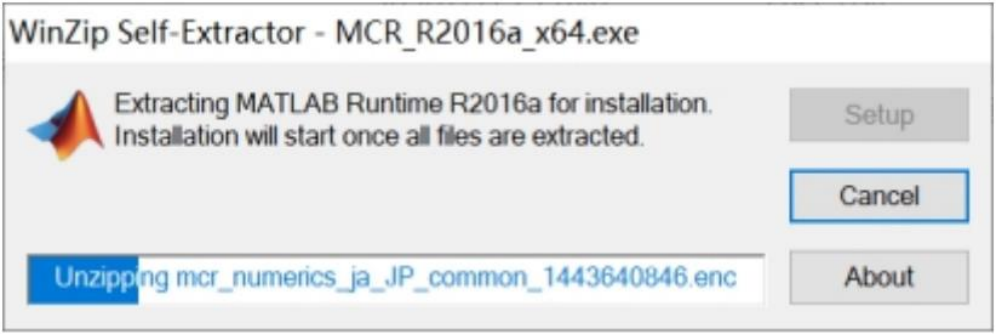
Figure 1-4-1
- Click Next, choose to agree to the terms, Next, click Install
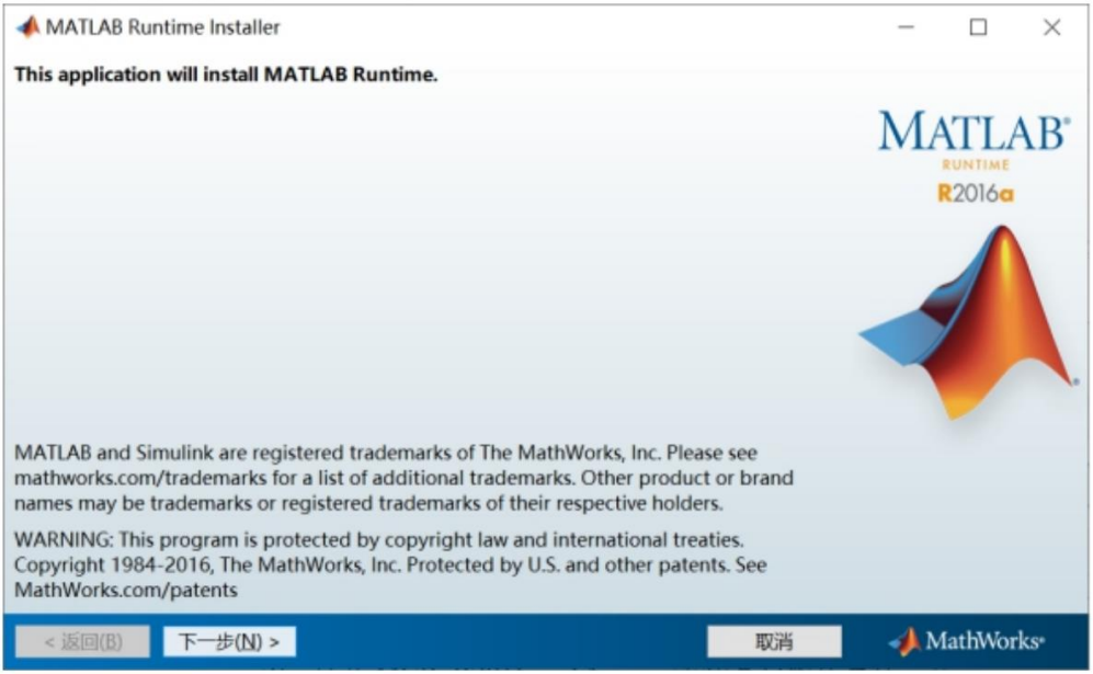
Figure 1-4-2
- Wait for the installation to complete
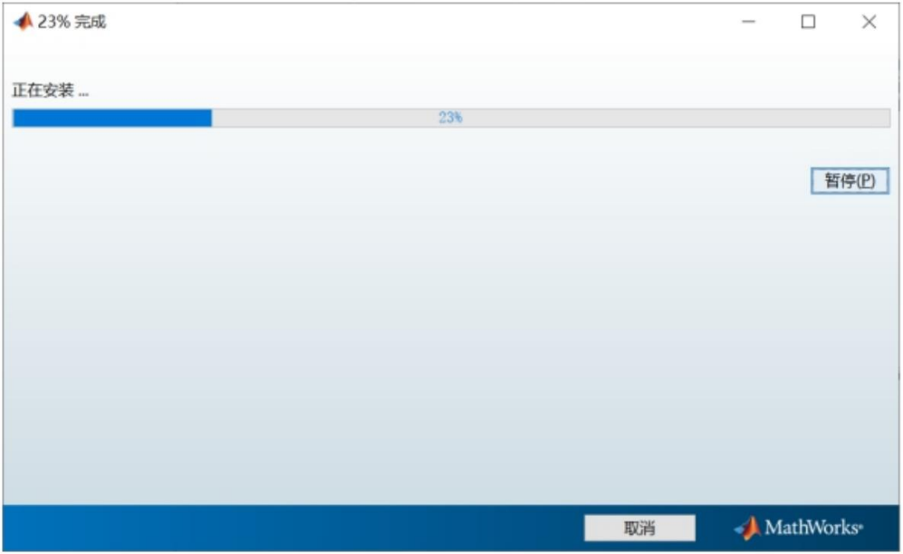
Figure 1-4-3
- Installation completed
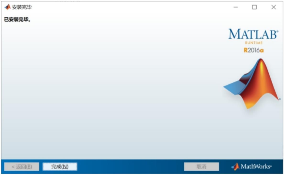
Figure 1-4-4
2 Function introduction
2.1 Overview
Users should follow the below process when doing the tuning work:
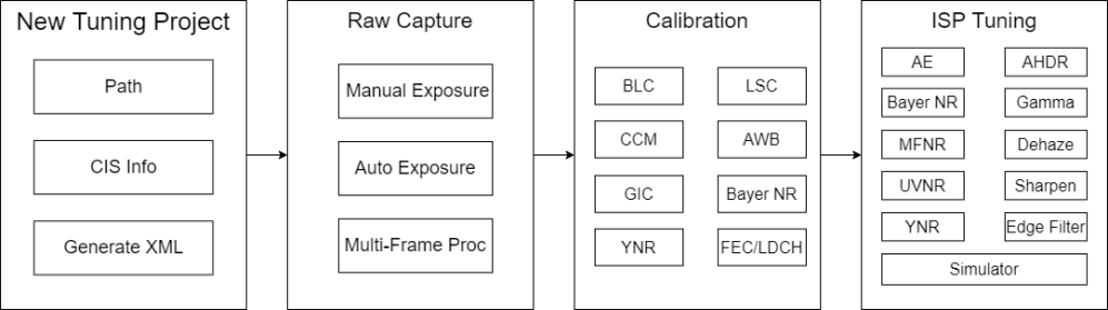
Figure 2-1-1
In the preparation stage, the user needs to generate a basic IQ file (.json format) in the tool, which records all the adjustable parameters in the ISP. After completing the tuning, the user needs to replace the file to the corresponding location in the firmware or device, and then restart the camera application to confirm the final image effect.
Since the functions of the tool such as raw capturing, online tuning, and parameter interaction are transmitted through the network protocol, therefore, when prepare for the tuning environment, users need to connect the PC and the device to the same local area network.
The calibration work should follow workflows as below:
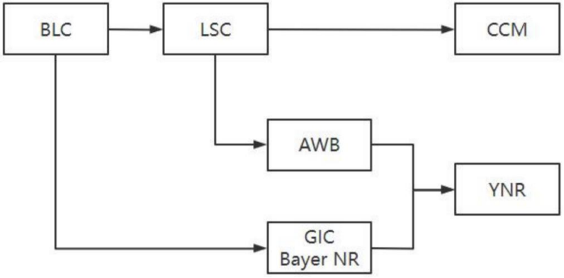
Figure 2-1-2
Since the calibration of some parts will depend on the results of previous one, users should complete the calibration work in the order of the process. After completing the calibration of one module, make sure the results are correct.
2.2 Sensor Configuration
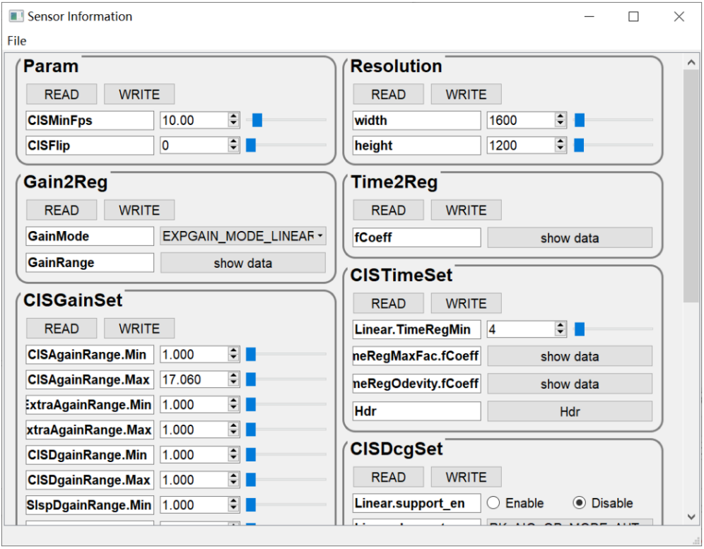
Figure 2-2-1
The Sensor configuration UI is shown in Figure 2-2-1. It has two parts:
- Parameter tuning area: For the parameter description please refer to the “sensorinfo parameters” in section 4.1.2.5 of Rockchip_Tuning_Guide_ISP21/30/32. Users should refer to the Sensor’s Datasheet to enter (this part may require the help of a driver engineer).
- Menu bar: Includes the import and export to SensorList.ini
2.3 RKISP Capture Tool
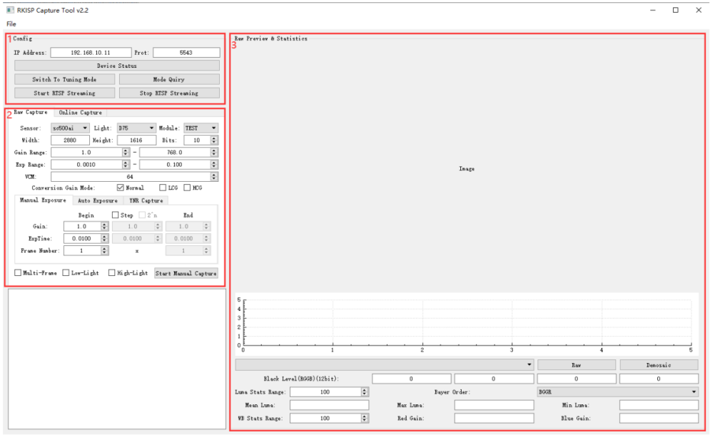
Figure 2-3-1
The main UI of RKISP Capture Tool is shown in Figure 2-3-1. It has 3 parts:
- Device-side connection configuration Provides device network parameter configuration, mode switching function, and test connection function.
- Capture settings It has two parts: Raw Capture and Online Capture: Raw Capture: Offline raw capture, including configuration of camera and exposure control: Configuration of Camera: Provides Sensor Exposure parameters, Source Name of Module/Light, Resolution and Gain/Exposure parameter ranges required for capture. Exposure control: Supports both manual exposure and automatic exposure, as well as a picture-taking function specially used for NR calibration. Manual exposure allows configuring the step size for traversing and capturing multiple exposure combinations. Automatic Exposure: This function is used to automatically search an exposure parameter until reaching the target brightness set by the user. YNR Capture: This function is used for capture a raw image for YNR Calibration, the detail please refers to chapter 4.6.1. Online Capture: This function is used for capturing in online stream, supports both raw and yuv formats.
- Preview and Statistics of Raw Images The captured Raw image (displayed in grayscale), histogram, and ROI brightness are displayed here.
2.4 RKISP Calibration Tool
The calibration tool will load the RKISP calibration tool (Figure 2-4-2) for the selected chip and version (Figure 2-4-1), and the imported IQ file should also match the chip and version.
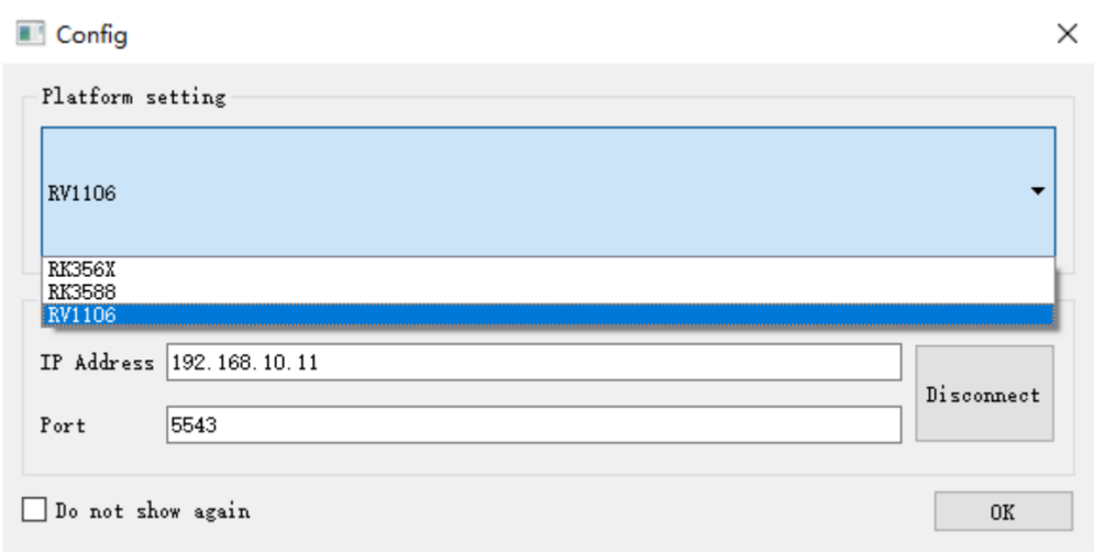
Figure 2-4-1
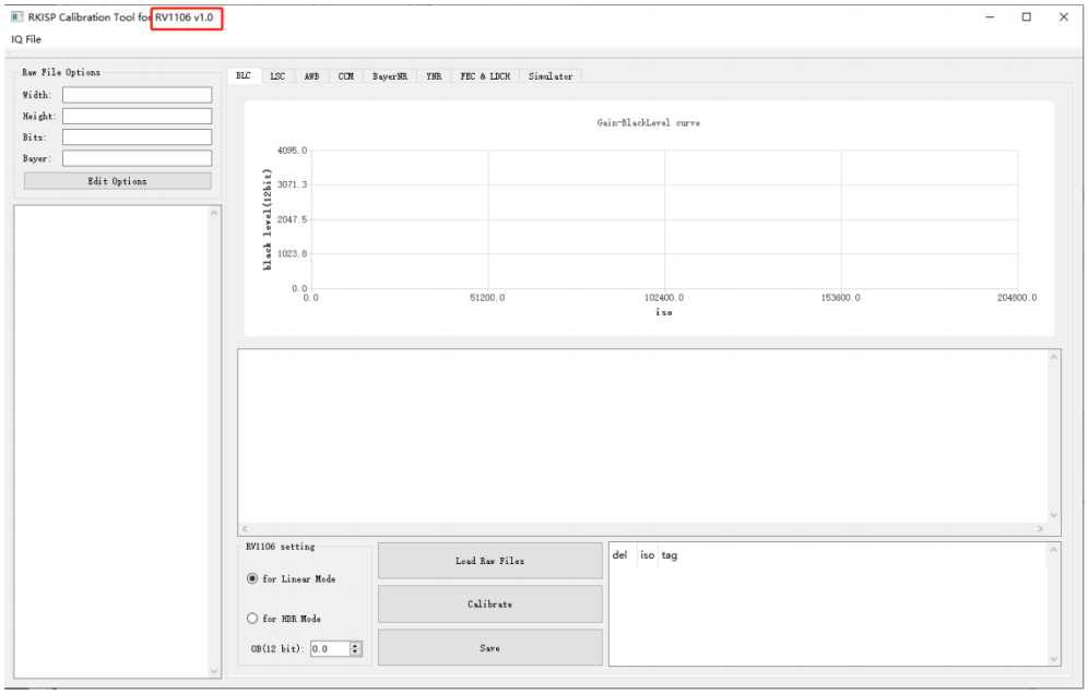
Figure 2-4-2
The main UI of RKISP Calibration Tool is shown in Figure 2-4-2, it includes the calibration functions of the following modules: BLC: Black Level Correction LSC: Lens Shading Correction CCM: Color Correction Matrix AWB: Automatic White Balance Correction
GIC: Green channel balance correction (calibration is integrated in the Bayer NR module) Bayer NR: Raw domain noise reduction, including Bayer 2DNR, Bayer 3DNR YNR: Y channel noise reduction FEC: Fisheye Calibration
2.5 RKRAW Tool
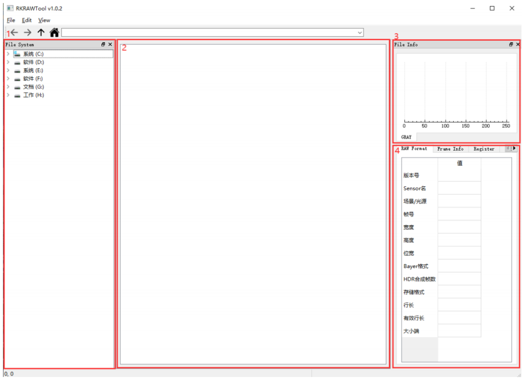
Figure 2-5-1
The main UI of RKRAW Tool is shown in Figure 2-5-1. It supports viewing in those formats: jpg/bmp/png, raw, RKRawV1, and RKRawV2. This tool has four parts:
- File system, for selecting the image path to view.
- Display window: Right-click the display area to switch between GRAY/RGB, Normal/Hdr Short/Mid/Long (only support the RKRawV2 format), as shown in Figure 2-5-2. Hold down the Ctrl and wheel in or out to zoom in or out.
- Histogram display: Histogram statistics in gray channel
- The information of RKRawV2: Such as raw format, exposure parameters, etc.
- Compare: Hold down the Ctrl and select more than 2 images at the same time and click compare button as shown in Figure 2-5-3.
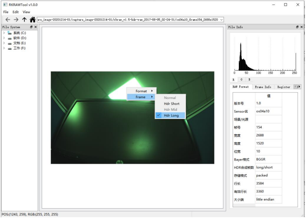
Figure 2-5-2
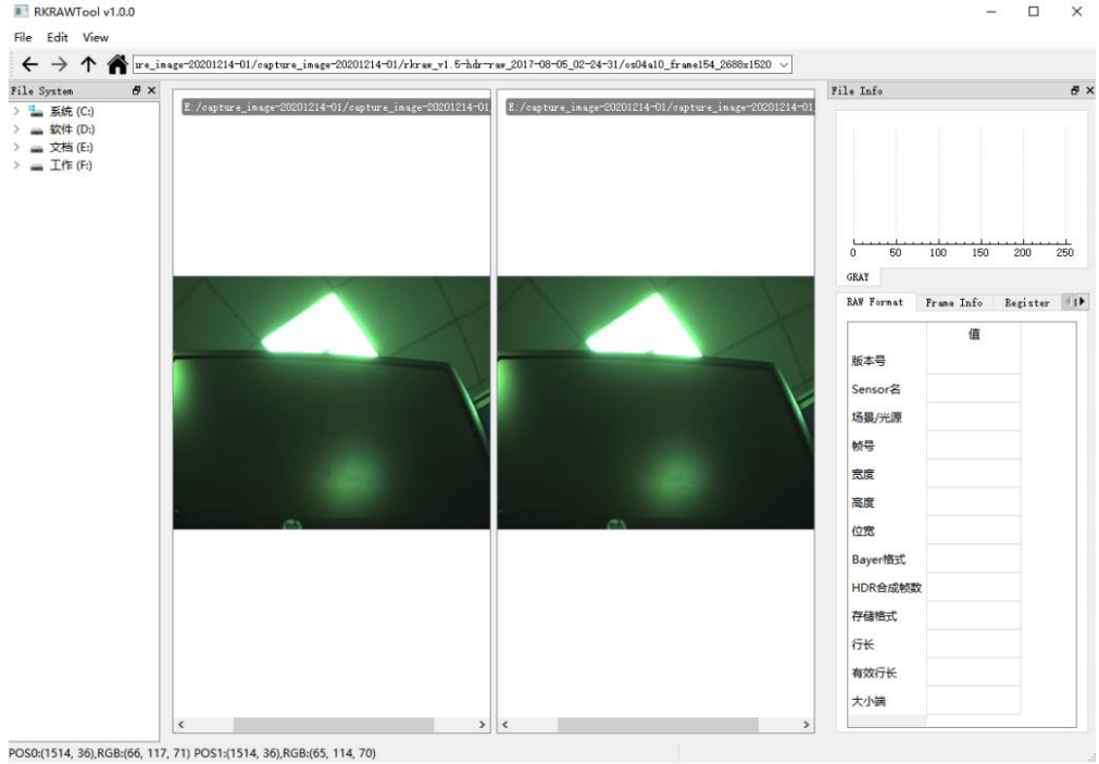
Figure 2-5-3
2.6 RKISP 3D-LUT Tools
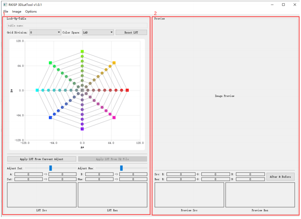
Figure 2-6-1
The main UI of RKISP 3D-LutTool is shown in Figure 2-6-1, including two parts: Left is the LUT area, right is the preview area.
- File: Includes image import, IQ parameter import and save, LUT Info import and save. Load Image: Click Load Image to import (supports jpg/bmp/png/nv12), the image will be displayed in the Preview area on the right as shown in Figure 2-6-2. Load IQ File: Click Load IQ File to import IQ parameters, select the scene and Lut3D table to be imported. As shown in Figure 2-6-3.
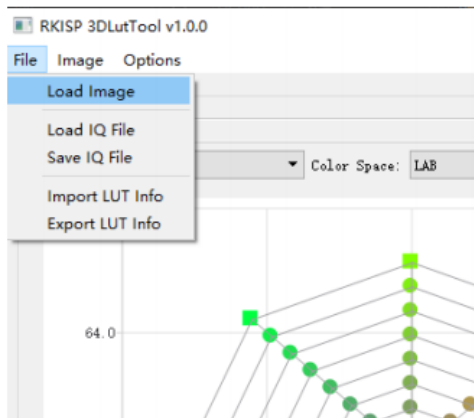
Figure 2-6-2
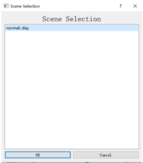
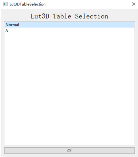
Figure 2-6-3
Save IQ File: Click Save IQ File, user can choose to overwrite an existing table in the IQ file or create a new table, as shown in Figure 2-6-4.
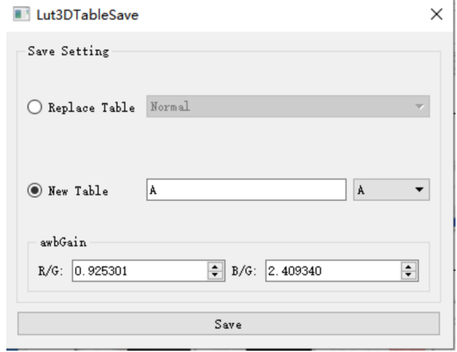
Figure 2-6-4
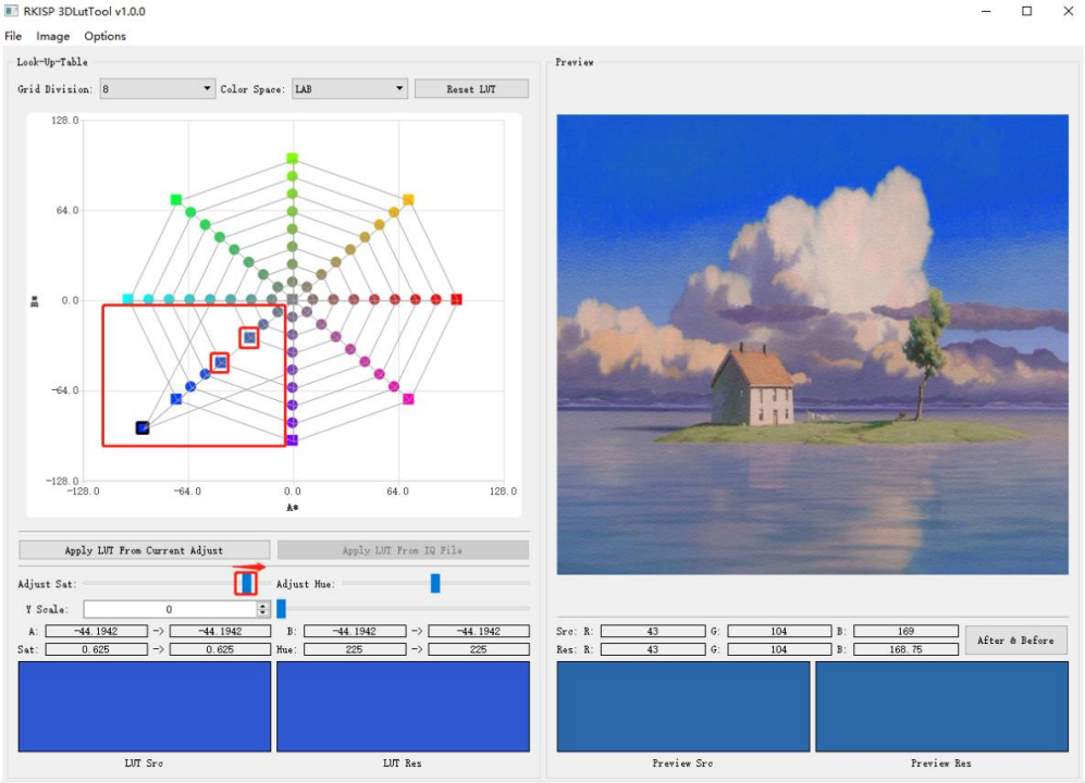
- Color search: Move the mouse on the image, the color corresponding to the mouse point will be marked in the left LUT, as shown in Figure 2-6-5. Left-click the current position to lock the marked color in the LUT. Adjust the color by “Adjust Sat” and “Adjust Hue” or directly drag the marked point. We can see the before and after of AB, Sat, Hue, RGB values of the marked points and the color changes in LUT/Preview.
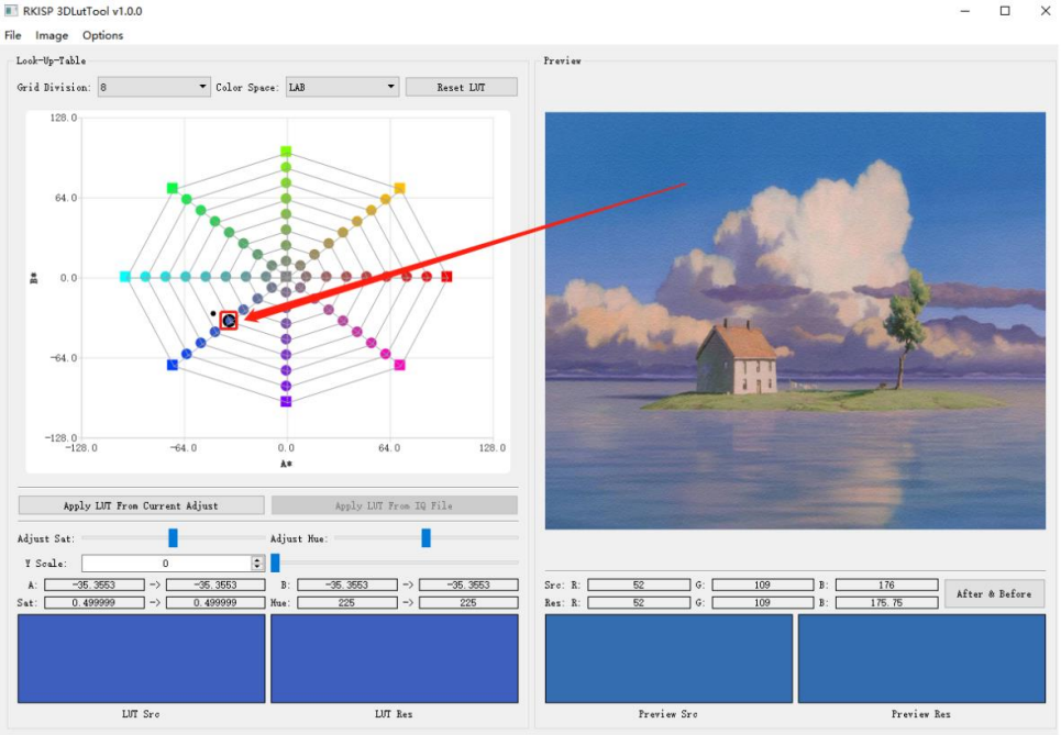
Figure 2-6-5
- Adjust Sat: Drag the slider, the marked colors in the LUT will change together with the nearest colors, as shown in Figure 2-6-6 (a). If you only want to change the marked color, and keep the positions of the other colors, you can right-click the color you don’t want to move, and after turning the dot into a square, its position is locked. Drag Adjust Sat, then only the marked color in the LUT changes. As shown in Figure 2-6-6 (b).
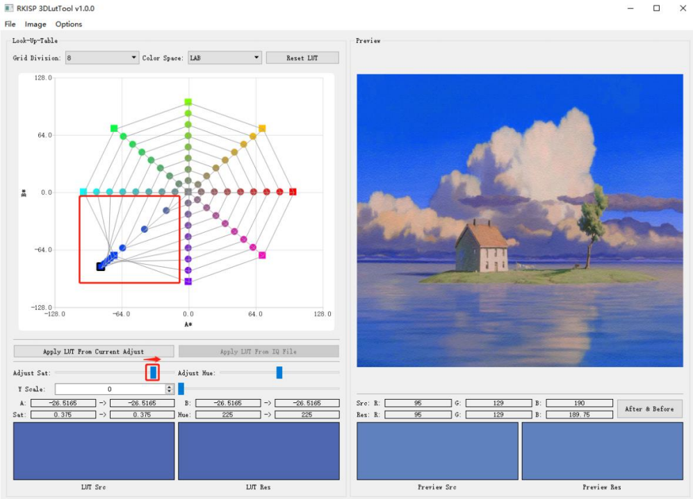
(a)
(b)
Figure 2-6-6
- After & Before: View the image before and after adjustment
- Reset LUT: Restore the default values of LUT
- Image: Support image left and right rotation, vertical/horizontal flip transformation and save the adjusted image, as shown in Figure 2-6-7
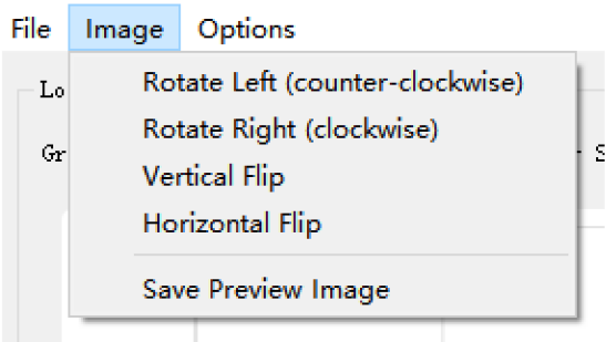
Figure 2-6-7
- Options: Support LUT display settings, you can adjust the size and line width of marker points, as shown in Figure 2-6-8.
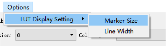
Figure 2-6-8
2.7 RKISP 3A Analyzer Tool
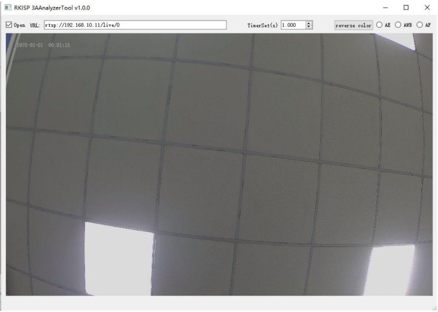
Figure 2-7-1
Click Connect to rkaiq_tool_server, open RKISP 3AAnalyzerTool, the main UI is shown as Figure 2-7-1, modify the URL address, check Open to start preview, the current version supports obtaining statistical data of AE and AWB modules.
TimerSet: Adjust the interval for getting data
Reverse color: Change the color of the data in the preview panel.
Click the AE button to open the AE module, and display the dynamic histogram in the AE Statistics window. Then the image in the preview panel of the main UI will be divided into 15 * 15 small grids, each grid will display the statistical value (12bit) of the corresponding block, the display channel can be switched by the Channel list, HDR mode supports L/M/S frame statistics display, as shown in Figure 2-7-2.
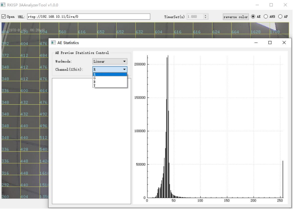
Figure 2-7-2
Click the AWB button. In the AWB Statistics window, the status information of the current AWB will be dynamically printed. Then the image in the preview panel of the main UI will be divided into 15 * 15 small grids, and each grid will display the number of white points and the WBGains of the corresponding block, as shown in Figure 2-7-3.
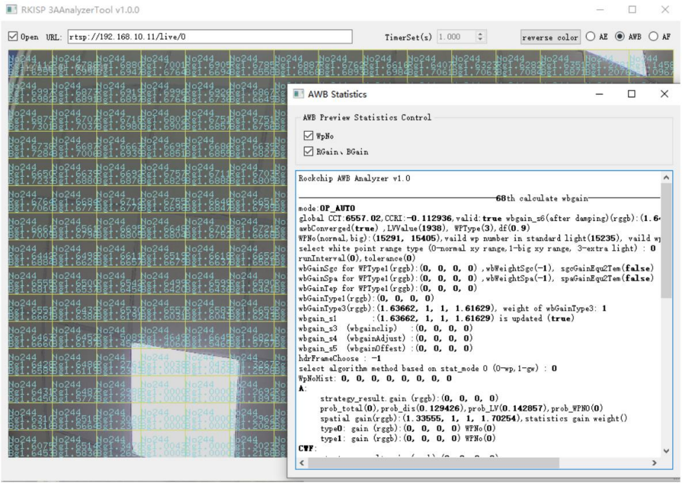
Figure 2-7-3
3 Quick Start
3.1 Preparations
The ISP tuning has a lot of work to do on the device side. Here we need to run a service application on the device side to transfer data between Tuner and AIQ, and we can also use it for capturing raw image and other works. To do this, before starting the Tuning job, the service application and other relevant files need to be push to the device and run. The following two parts describe the preparations required to tuning on the Android and Linux:
- LAN connection
- Run rkaiq_tool_server and other environment configuration jobs (where command execution and file transfer can be done via: TFTP, serial port, ADB and other protocols or tools. ADB is used in the example)
3.1.1 Android
3.1.1.1 RK356X & RK3588
For devices that can be connected using a wired network:
- Connect the device to the router with a network cable
- Use the ifconfig command to view the IP address of the device
- The PC is also connected to the same router (either wired or wireless)
- Check the IP address of the PC, and use ping on the command line of the PC or device to confirm that the network path is normal
For devices that cannot be connected using a wired network (tablets, etc.):
- Connect the PC and EVB with a USB cable (the same port as ADB)
- Turn on the power and enter the system
- Open Settings
- Enter Network&internet
- Enter Hotspot&tethering
- Turn on USB tethering
- adb shell into the device side
- Execute ifconfig usb0 to view the IP address
- Use ping on the command line on the PC or device side to confirm that the network path is normal
Operations required to run rkaiq_tool_server (if the required service application and other dependent files already exist in the corresponding path on the device side, just run rkaiq_tool_server directly):
- Compile and obtain rkaiq_tool_server and rkaiq_3A_server in the SDK
- Path in SDK: external/rkaiq_tool_server, firmware must be user-debug version
- Push the android.hardware.camera.provider@2.4-service.rc file into /vendor/etc/init/ on the board under the path
- Enter the /vendor/etc/init/ path and execute the command to modify permissions: chmod 644 android.hardware.camera.provider@2.4-service.rc
- Push rkaiq_tool_server and rkaiq_3A_server into the /vendor/bin/ path of the board
- Enter the /vendor/bin/ path and execute the command to modify permissions: chmod 755 rkaiq_tool_server (and rkaiq_3A_server)
- Execute the flush cache command: sync
- Restart the device
- Execute the command: setenforce 0
- Open the camera apk
- Run rkaiq_tool_server
Example of ADB operation:
#The following commands are run in cmd on the PC side
adb root
adb remount
adb push android.hardware.camera.provider@2.4-service.rc /vendor/etc/init/
adb push rkaiq_tool_server /vendor/bin/
adb shell

# The following commands are executed in adb shell terminal
chmod 644 /vendor/etc/init/android.hardware.camera.provider@2.4-service.rc
chmod 755 /vendor/bin/rkaiq_tool_server
sync
reboot

# After restart, enter adb shell again
# disable SELinux
setenforce 0
# Manually run the camera apk first
# Then run tool server
/vendor/bin/rkaiq_tool_server &
For multiple cameras example:
#If there are 2 sensors in the device and you need to switch to another sensor for tuning, run tool server as follows:
/vendor/bin/rkaiq_tool_server -d 1 &
Note: After pushing the initial version of IQ parameters generated by the “New” function into the device, use the following operations to reset the camera application and run ToolServer again. If there are abnormal problems such as crash, stuck, failure of online tuning, unable to preview, etc., please also try to reconnect the tool according to the following steps
source /vendor/etc/camera/reset_camera.sh
# run camera apk
/vendor/bin/rkaiq_tool_server &
3.1.2 Linux
3.1.2.1 RK356X & RK3588 & RV1106
For devices that can be connected using a wired network:
- Connect the device to the router with a network cable
- Use the ifconfig command to view the IP address of the device
- The PC is also connected to the same router (either wired or wireless)
- Check the IP address of the PC, and use ping on the command line of the PC or device to confirm that the network path is normal
For devices that cannot be connected using a wired network:
- Try to start the RNDIS service
- Use the ifconfig command to view the IP address of the device
- Use ping on the command line on the PC or device side to confirm that the network path is normal
Operations required to run rkaiq_tool_server (if the required service application and other dependent files already exist in the corresponding path on the device side, just run rkaiq_tool_server directly):
- Compile and obtain rkaiq_tool_server and librkmedia.so in the SDK
- Push the librkmedia.so file into the /data/ path of the board
- Enter the /data/ path and execute the modify permission command: chmod 777 librkmedia.so
- Push the rkaiq_tool_server file into the /data/ path of the board
- Enter the /data/ path and execute the modify permission command: chmod 777 rkaiq_tool_server
- Execute the flush cache command: sync
- Restart the device
- Run the camera app
- Run rkaiq_tool_server
Example of ADB operation:
#The following commands are run in cmd on the PC side
adb root
adb remount
adb push librkmedia.so /data/
adb push rkaiq_tool_server /data/
adb shell

# The following commands are executed in adb shell
chmod 777 /data/rkaiq_tool_server
sync
reboot

# After restart, enter adb shell again
# Run the camera app first
/data/rkaiq_tool_server &
3.2 ToolServer Parameter Instructions
Here is a brief description of the parameters and configurations of rkaiq_tool_server:
-d: sensor selection, when there are multiple sensors in the device that need to be tuned, you can use the device number such as 0/1/2 to select which sensor to use. The default value is 0. For the query method of the specific device number, refer to the following description: media-ctl -p -d /dev/mediaX (X=0/1/2/3…) The output will have a topology structure, and the nodes in it contain the sensor name, for example: “m01_b_ov8858 2-0036”, m01 corresponds to mNN , NN is a 2-digit sensor index, then the parameter configuration is -d 1, 1 corresponds to the above NN, less than 2 digits do not need to add 0 in front
-s: Select the video node for YUV capture. The default value will automatically search for the iqtool node, or it can be manually specified to mainPath or selfPath
-r: RTSP switch, 0 is off, 1 is on, the default value is 0, you can use the Start RTSP function in CaptureTool after it is turned on
-i: IQ file path, if the path is changed, this parameter should be modified synchronously, it can be ignored when the -r parameter is 0
-w/-h: Configure RTSP video stream preview output resolution, the resolution will be scaled based on ISP output size to meet the requirements, the default value is 1920/1080
-n: The number of buffers used for online capture of continuous Raw, the default value is 4, it is recommended to increase this parameter when you need to capture a large number of continuous Raw images
-f: The sending frame rate of the offline frame function, the default value is 10 frames
3.3 Platform Setting & IP Address
- Open RKISP Tuner, the initial configuration window as shown in Figure 3-3-1.
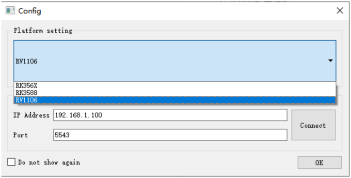
Figure 3-3-1
- Select the chip, enter the IP address obtained in the previous section, the port number is 5543 by default (do not modify it unless there are special requirements), please make sure that rkaiq_tool_server is running correctly, click Connect to rkaiq_tool_server, after the connection, if need to use third-party tools to preview, please refer to the point 3 of chapter 3.7 for specific operations.
- Click OK, the tuning UI of the selected chip and version as shown in figure 3-3-2.
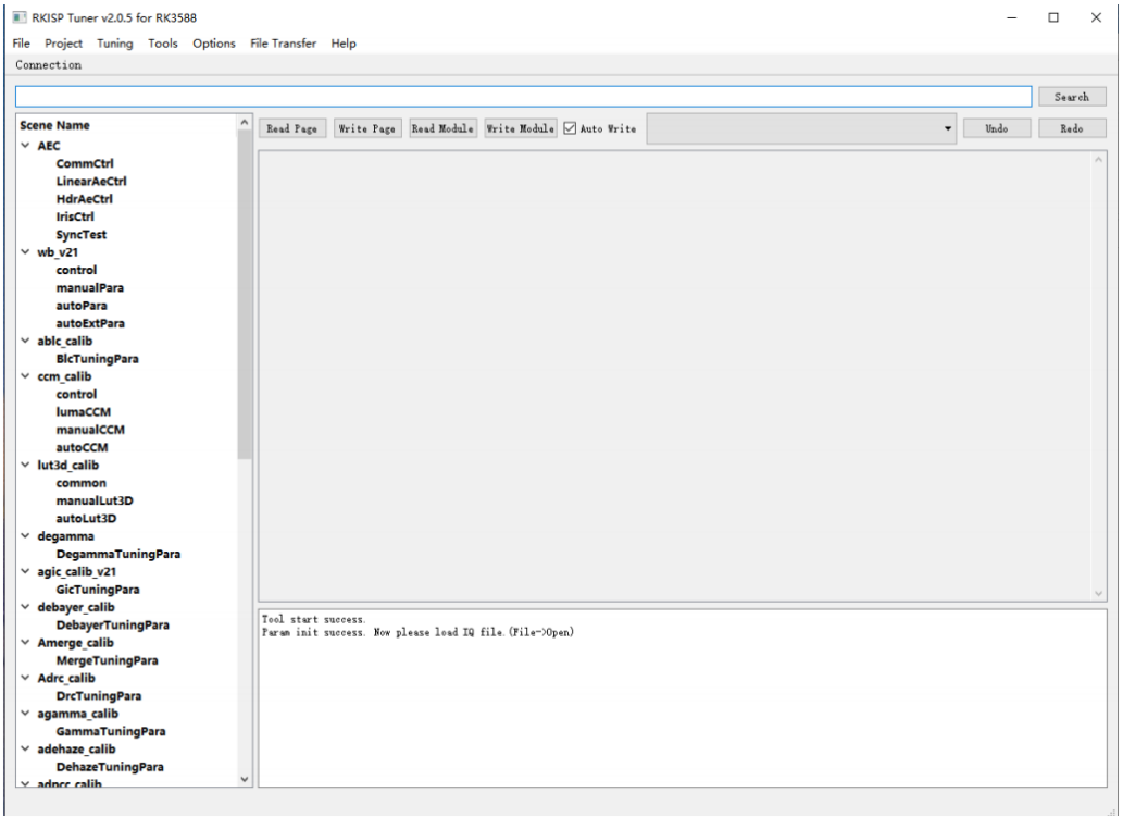
Figure 3-3-2
3.4 Generate New Sensor Configuration and IQ File
- Click the “File” - “New” buttons.
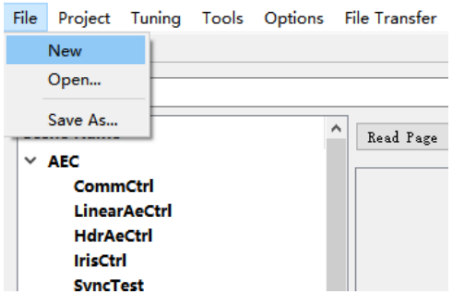
Figure 3-4-1
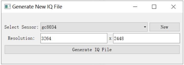
Figure 3-4-2
- Click the “New” button on the right side of the Sensor list to open the Sensor Information page.
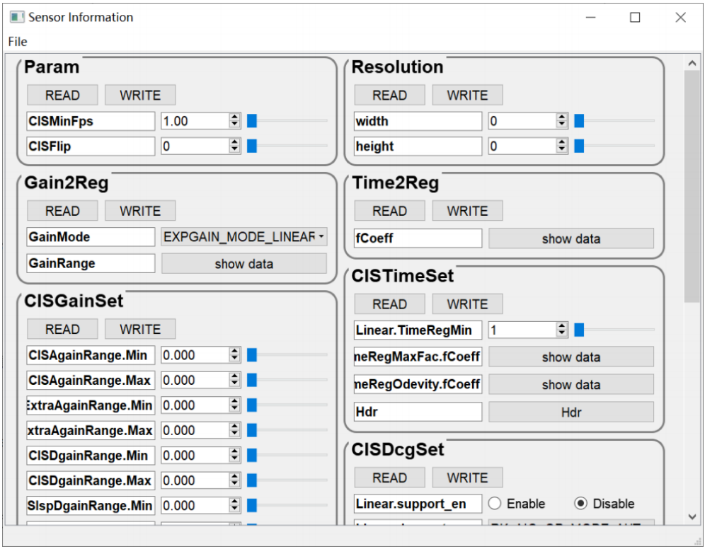
Figure 3-4-3
- After filling in the Sensor Information, click the button “File” - “Export To Sensor List”.
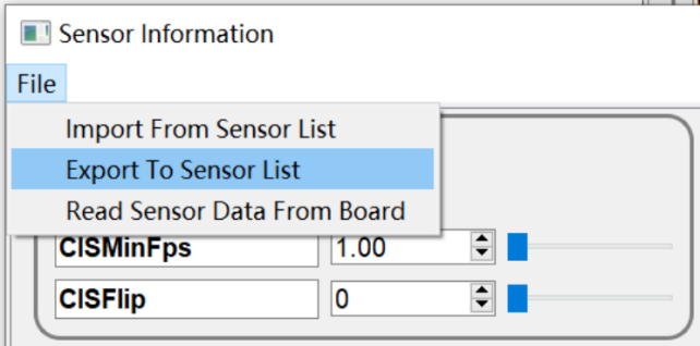
Figure 3-4-4
- Enter the saved Sensor name and click “OK” to save the configuration.
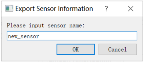
Figure 3-4-5
- Close the configuration page, we can see the new Sensor name in the Sensor list on the Generated New IQ File window.
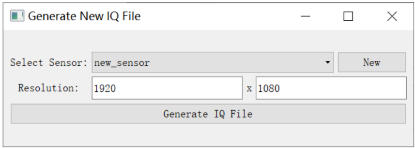
Figure 3-4-6
- Select the Sensor and click the “Generate IQ File”, an IQ file is generated.
3.5 Load and Save Parameters & Scene Selection
- Click the “File” - “Open…” and select the IQ file you want to load.
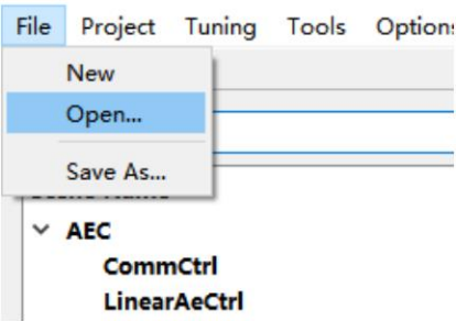
Figure 3-5-1
- In the Scene Selection window, the name of each group of scenes in the IQ file will be displayed, select the scene you want to tune, and click OK.
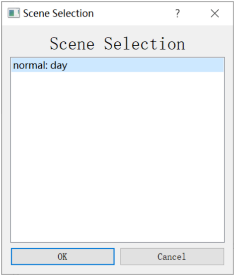
Figure 3-5-2
- At this point, the IQ file will be compared with the UI template parameters, their differences will be in the Different Member List. The list on the left shows the Missing parameters in the IQ file, and the list on the right shows the Existed parameters in the IQ file but have been removed or renamed in the UI template;
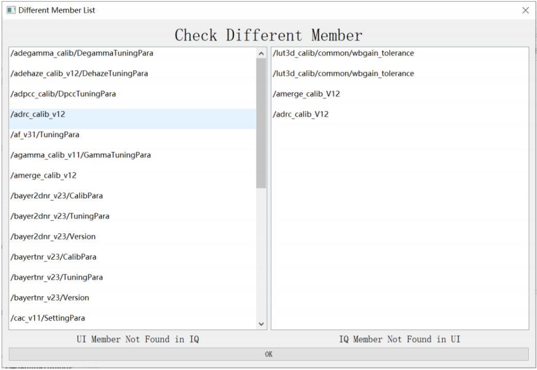
Figure 3-5-3
- Click “File” - “Save As…”, as shown in Figure 3-5-4 and 3-5-5, we can save the parameters to the scene parameters selected in step 2, or save as a new scene parameter, support saving only selected modules parameters, and display the modified parameters in the list on the right for reference.
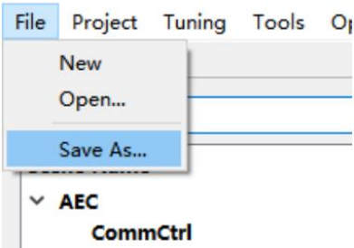
Figure 3-5-4
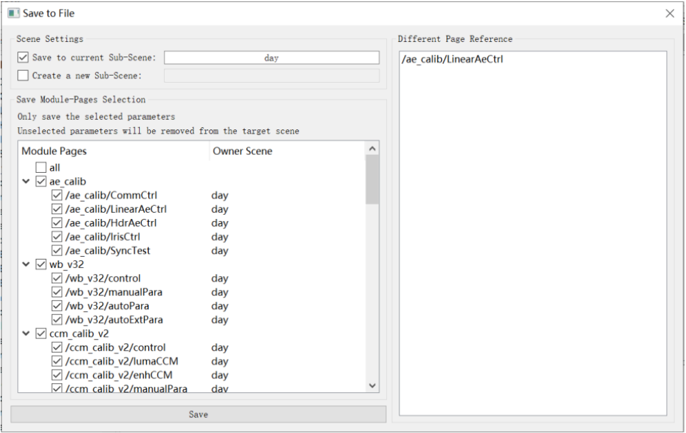
Figure 3-5-5
3.6 Edit Sensor Information
- Refer to the steps in the previous section to load an IQ parameter file.
- Click “Tuning” - “Edit Sensor Information” to open the Sensor Info configuration interface.
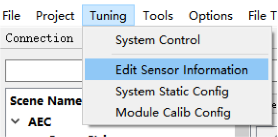
Figure 3-6-1
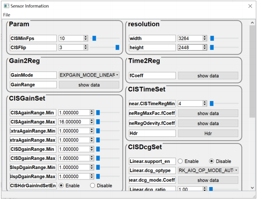
Figure 3-6-2
- Click “File” - “Import From Sensor List”.
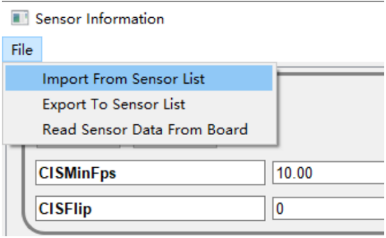
Figure 3-6-3
- Select the Sensor as shown below:
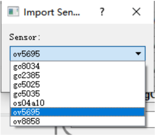
Figure 3-6-4
- Click “OK” to import the configuration parameters.
- Close the “Sensor Information” window.
- When the sensor name cannot be found in the sensor list, the user can refer to the sensor data sheet to create a new configuration in the Sensor Information window.
3.7 Capture Raw and YUV Images
3.7.1 Capture Raw Image Offline
- Click the “Tools” - “RK Capture Tool”.
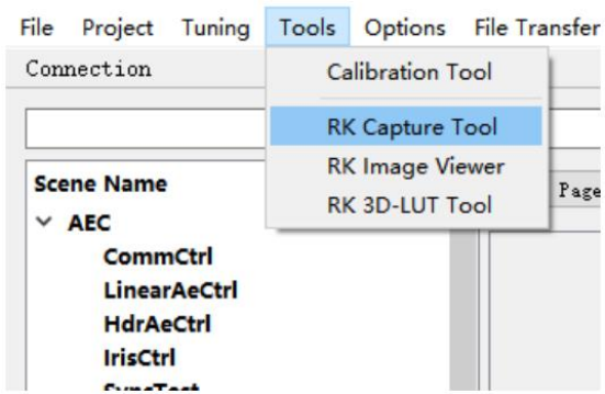
Figure 3-7-1-1
- Make sure the device IP address is entered correctly, click the “Device Status” button, if the Tuner is connected with rkaiq_tool_server correctly, it will print “Device is Ready”
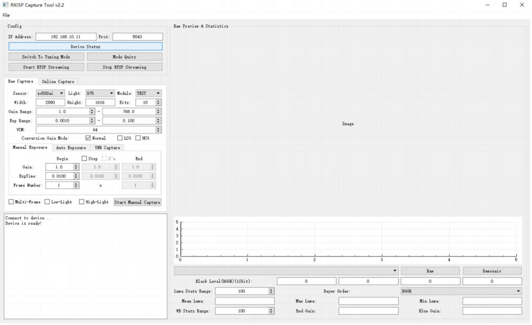
Figure 3-7-1-2
- Click Start RTSP Streaming to turn on the camera and start RTSP video streaming (optional)
1) Android: After clicking Start RTSP Streaming, you can use a third-party playback tool to open rtsp://192.168.10.104:1234/v to preview. At this time, the camera apk on the device will be disconnected, if you want to use the camera, please click Stop RTSP Streaming first, and then click Switch To Tuning Mode to open the camera.
2) Linux: If there are other camera devices running on the board, exit it and then run ToolServer. After clicking Start RTSP Streaming, you can directly use a third-party playback tool to open rtsp://192.168.10.104/live/0 to preview it.
- Select the name of sensor to tuning.
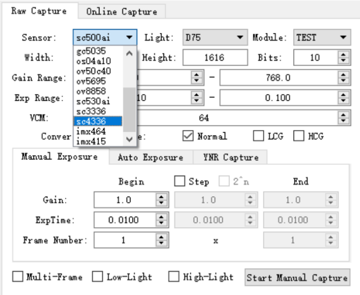
Figure 3-7-1-3
- Choose the correct resolution, light source and module name to distinguish in use.
- Configure parameters such as Gain, Exposure Time and number.
- Click the Start Manual Capture button.
- The captured raw image will be in the Raw Preview & Statistics on the right side.
- The histogram information, maximum/minimum/average brightness, global wb gain, etc. can also be found here.
- Raw images are stored in ./raw_capture/module name/ by default.
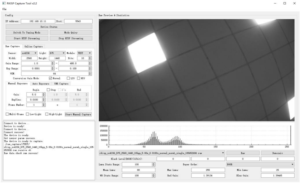
Figure 3-7-1-4 Captured a single-frame raw image with Gain=5x ExpTime=0.01s
3.7.2 Capture YUV Image Online
- Open the camera app and make sure the preview of the device work correctly.
- Run ToolServer, enter the IP address of the tool and connect to the device.
- Switch to the Online Capture, enter the name in Sensor Name, it will become the prefix of the YUV file name.
- When we need to capture continuous frames , configure the number in Frame Num.
- Click Capture YUV, the image can be previewed, the file will be stored in raw_capture/yuv/, as shown in Figure 3-7-2-1:
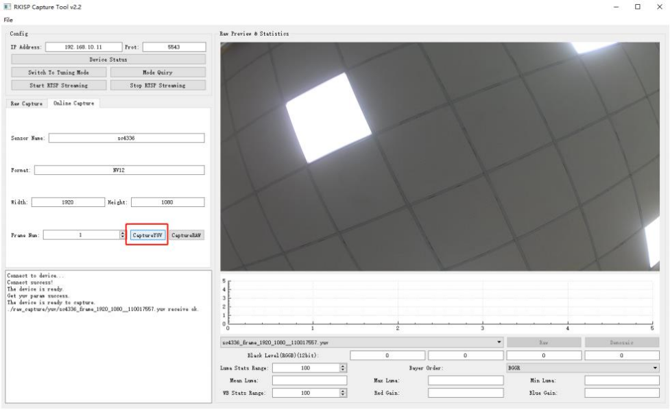
Figure 3-7-2-1
3.7.3 Capture Raw Image Online
- Open the camera app and make sure the preview on the device works
- Run ToolServer, enter the IP address in the tool side, and connect to the device
- Switch to the Online Capture, enter the name in Sensor Name, it will become the prefix of the Raw file name
- When we need to capture continuous frames , configure the number in Frame Num
- Click Capture Raw, the image can be viewed on the preview, the file will be stored in raw_capture/, as shown in Figure 3-7-3-1:
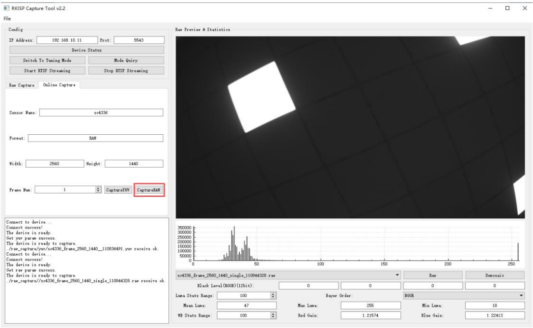
Figure 3-7-3-1
About the maximum number of consecutive frames for capturing Raw online
The maximum number of consecutive frames depends on the number of cache buffers applied for. This parameter can be configured through the -n parameter of ToolServer. The larger the number of buffers, the more consecutive frames can be captured in one performance. When the number of buffers is less than the number of captured frames, frames may be dropped. The number of buffers that can be configured also depends on the number of caches and memory size allocated by the kernel. For the kernel part, please refer to the following example:
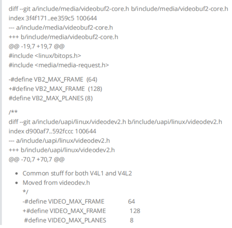
The patch image is fully transcribed below; the original remains for comparison. This is a source fragment, not a patch guaranteed to apply to an arbitrary kernel.
diff --git a/include/media/videobuf2-core.h b/include/media/videobuf2-core.h
index 3f4f171..ee359c5 100644
--- a/include/media/videobuf2-core.h
+++ b/include/media/videobuf2-core.h
@@ -19,7 +19,7 @@
 #include <linux/bitops.h>
 #include <media/media-request.h>

-#define VB2_MAX_FRAME (64)
+#define VB2_MAX_FRAME (128)
 #define VB2_MAX_PLANES (8)

 /**
diff --git a/include/uapi/linux/videodev2.h b/include/uapi/linux/videodev2.h
index d900af7..592fccc 100644
--- a/include/uapi/linux/videodev2.h
+++ b/include/uapi/linux/videodev2.h
@@ -70,7 +70,7 @@
 /*
  * Common stuff for both V4L1 and V4L2
  * Moved from videodev.h
  */
-#define VIDEO_MAX_FRAME        64
+#define VIDEO_MAX_FRAME        128
 #define VIDEO_MAX_PLANES       8
4 Descriptions of Calibration
The calibration work of each module has three parts:
- Capturing the images: According to the needs of each module, use the appropriate exposure to capture the raw image of the calibration board or scene.
- Calculate calibration parameters: import raw images, calculate calibration parameters, and individual modules can fine-tune some parameters as needed.
- Confirm and save the parameters: according to the standards of each module, judge whether the calibration parameters are correct.
4.1 Capture Raw Images
Refer to the operation steps in Section 3.6.
4.2 BLC Calibration
4.2.1 Basic Principles
Since the sensor has Black Level, it also has a certain output voltage when there is no external light, and the final output of the sensor needs to be subtracted from this value. In order to measure this value, some pixels that are not exposed at all are reserved. By reading the size of these pixel values, the Optical Black Level can be obtained in real time. At this time, the output of the sensor is: Raw = Sensor Input - Optical Black Level
In addition, considering the signal-to-noise ratio of the sensor output, a base Pedestal is usually placed on the sensor output, and the output at this time is: Raw = Sensor Input - Optical Black Level - Pedestal
Due to the different sensor configurations, for the BLC module, the final BLC correction value can be obtained by capturing the RAW data in the complete black scene.
The correction value here is mainly affected by Gain and Temperature, so it needs to be calibrated separately at different ISOs. Since BLC is an offset, other modules need to deduct the offset when calibrating, otherwise the correct calibration parameters cannot be obtained.
RV1106 platform: In order to retain more dark information during Bayer2D and Bayer3D noise reduction, the BLC module adds Sensor OB configuration, which is the Pedestal mentioned above. Some manufacturers support the configuration in the driver sequence, Some are fixed values, which can
be confirmed by querying the data sheet or the driver code. If it is difficult to confirm the value, you can use the reference value in Section 4.2.4 or the BLC average value of each channel calculated by using Gain=1x.
4.2.2 Raw Image Requirements
- Cover the lens when capturing, make sure no light enters.
- Capturing needs to traverse Gain=1x, 2x, 4x, 8x, 16x…Max (if the driver supports the maximum Gain to 40x, then Max=32).
- The exposure time does not affect the BLC calibration and can be unified to 10ms.
4.2.3 Capture Raw Image
- Open the RK Capture Tool, refer to the instructions in Sections 3.1 and 3.2, connect to the device, select unknow (no light) for the light source name, and BLC for the module name.
- Put the device or module in a no light environment, and use a black cloth, lens cover, etc. to cover the lens tightly.
- Check Step and 2^n on the Manual Exposure page, according to Gain Range, configure: Gain Begin=1.0 and Gain End=Max, and ExpTime=0.010.
- Click Start Manual Capture to capture the Raw image in steps of 2 to the Nth power.
- The captured Raw image will be displayed on the right side, select the image you want to view by switching the drop-down box.
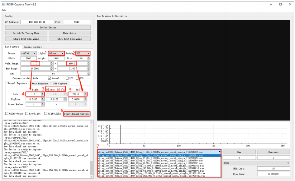
Figure 4-2-3-1
4.2.4 Calibration Procedure
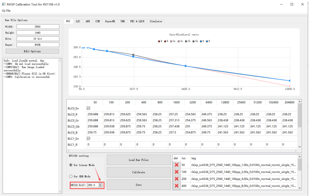
Figure 4-2-4-1 BLC calibration results
- Open Calibration Tool, click Edit Options in the upper left of the interface, open the configuration interface, and enter the size, bit width and bayer order of the raw image.
- Select the BLC page, click the Load Raw Files, and select a folder to store Raw images.
- The imported Raw image will be displayed in the list on the right.
- Click Calibrate to start. RV1106 platform: Linear mode calibration needs to enter the Sensor OB value first. We list some commonly used OB values for reference:
| Manufacturers | OB value for reference |
|---|---|
| GalaxyCore(gc) | 256 |
| OmniVision(ov/os) | 256 |
| Samsung(s5k) | 256 |
| SmartSens(sc) | 256 |
| Sony(imx) | The driver sequence can be configured, it is recommended to refer to the DataSheet and driver code, whichever is the actual. |
- The Black Level Curve obtained from calibration is displayed on the upper axis.
- The BLC value obtained from calibration will be in the table, click Save. Notes:
- If the device itself has power light and status indicators, etc., pay attention to whether there is light leakage.
- An incorrect BLC value will affect the calibration results of all subsequent modules. Please make sure that the BLC results are correct before performing subsequent calibration.
4.3 LSC Calibration
4.3.1 Basic Principles
Luma Shading is caused by the optical properties of the lens. For the entire lens, think of it as a convex lens. Since the light-gathering ability of the center of the convex lens is much greater than that of its corner, the light intensity in the center of the Sensor is greater than that in the corner areas. For an undistorted camera, the illumination attenuation around the image follows the formula:
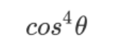
cos^4(theta)
4.3.2 Raw Image Requirements
- When capturing, cover the lens with diffuser (or use DNP light box, integrating sphere and other equipment).
- Capture in a light box with standard lighting, we recommend to calibrate 7 light sources: HZ, A, CWF, TL84, D50, D65, D75.
- To prevent the AC light source from generating Flicker, it is recommended to use an integer multiple of 10ms to configure the exposure time.
- The maximum brightness of the Raw image is about 200 (8bit), and the minimum brightness should be significantly larger than the black level value calibrated in the previous section.
- We recommend to use the diffuser as shown below:
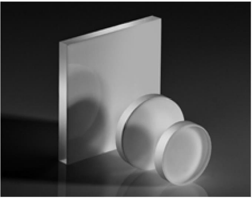
Figure 4-3-2-1 Opal Diffuser
4.3.3 Capture Raw Image
- Open the RK Capture Tool, refer to the instructions in sections 3.1 and 3.2, connect to the device, and select LSC as module name.
- Put the module in the light box, switch to HZ light, and place the diffuser close to the lens.
- Select HZ light source, check Search Exposure by Max Luma (8bit) on the Auto Exposure page, check Anti Flicker (50hz), and configure the maximum brightness of the target over the right to 200±10%, Frame Number = 1.
- Click Start Auto Capture to capture a raw image, during which the tool will automatically select the appropriate exposure until it meet the preset maximum brightness.
- Switch the light source to A, change the name of the light source to A, and repeat step 4 until all light sources are finished.
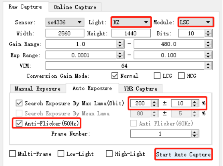
Figure 4-3-3-1
4.3.4 Calibration Procedure
- Open Calibration Tool, click the Edit Options in the upper left corner, open the configuration interface, and enter the size, bit width and bayer order of the raw image.
- Select the LSC and click the Load Raw Files to import all raw images.
- The imported raw image will be displayed in the above window.
- Modify the Light Fall off to 100%.
- Click Calibrate to start.
- After calibration is done, we can view the raw image of each light source on the result page.
- Click Save.
- Modify the Light Fall off to 70%, repeat steps 5~7.
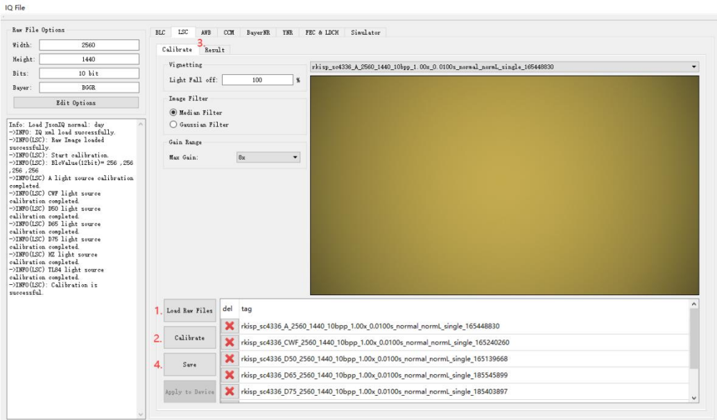
Figure 4-3-4-1
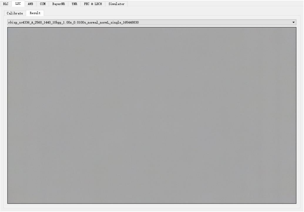
Figure 4-3-4-2
Notes: The tool may not be able to find suitable exposure parameters because the light is too bright or too dark. In this case, we can refer to the following solutions:
- Adjust the brightness of the light source.
- Use ND filter.
- Adjust the lens orientation.
- Modify the Gain Range or Exp Range.
- Adjust the maximum brightness or threshold value for automatic exposure.
- Use manual exposure instead (the minimum standard for selection is that the minimum brightness is significantly greater than the Black Level value calibrated in the previous section).
4.4 AWB Calibration
4.4.1 Introduction
Calibrate the white point conditions of raw in XY, UV, YUV, the simple color algorithm parameter and the white balance gain under standard light source.
4.4.2 Raw Image Requirements
Preparations for capturing raw images:
- Equipment: X-Rite 24 ColorChecker, Light Box (including D75, D65, D50, TL84, CWF, A, HZ)
- Adjust the exposure parameters, so that the maximum value of the brightest white block in the color is [150-240], the brighter the better within this range (if you want to use the same raw image with the following CCM, it should be darker)
- The ColorChecker occupies more than 1/9 of the screen Raw image capturing method:
- Open the RK Capture Tool, refer to chapter 3.1 and 3.2, connect to the device, module selects to CCM_AWB.
- Put the device and the ColorChecker in the light box, adjust their position, make the ColorChecker in the center of the screen, capture as large as possible, and do not move the device
- Open the light box and switch the light source to HZ light.
- Select HZ, check Search Exposure By Max Luma (8bit) on the Auto Exposure page, check Anti Flicker (50hz), and configure the maximum brightness of the target on the right to 200±10%, Frame Number = 1. (If at 1x Gain, 10ms integer multiples cannot capture raw images, turn off Anti-Flicker (50hz) and try again)
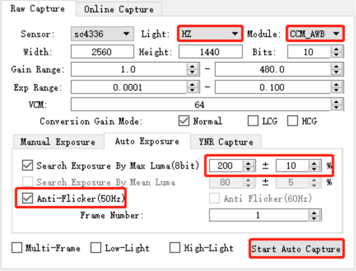
Figure 4-4-2-1
- Click Start Auto Capture, the tool will automatically select the appropriate exposure until the preset maximum brightness is reached.
- Switch the light source to A, name the light source to A, and repeat the previous steps until all light sources are finished.
For example, the calibration raw image after demosaicing are as follows:
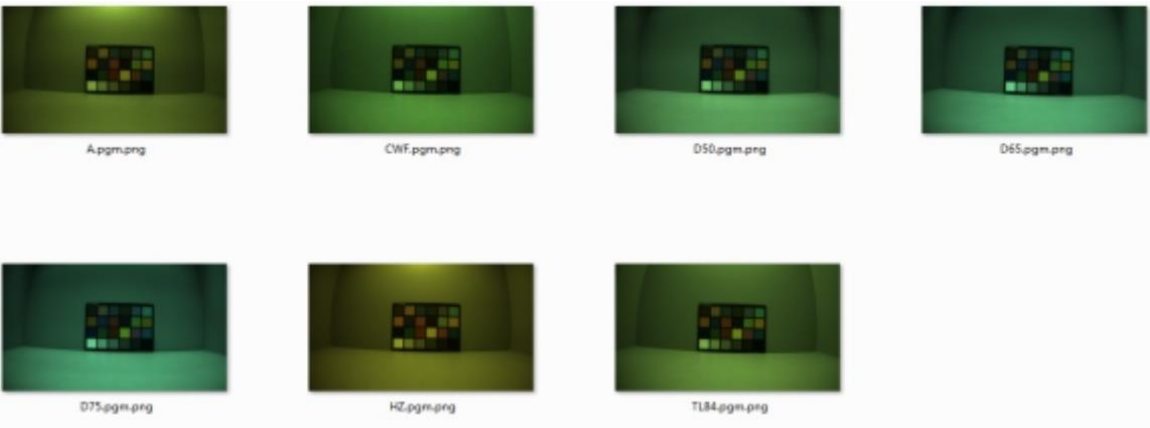
Figure 4-4-2-2
4.4.3 Calibration Tool Introduction
- Adjust the white point condition of the UV and XY domains, and the TH value of the YUV domain.
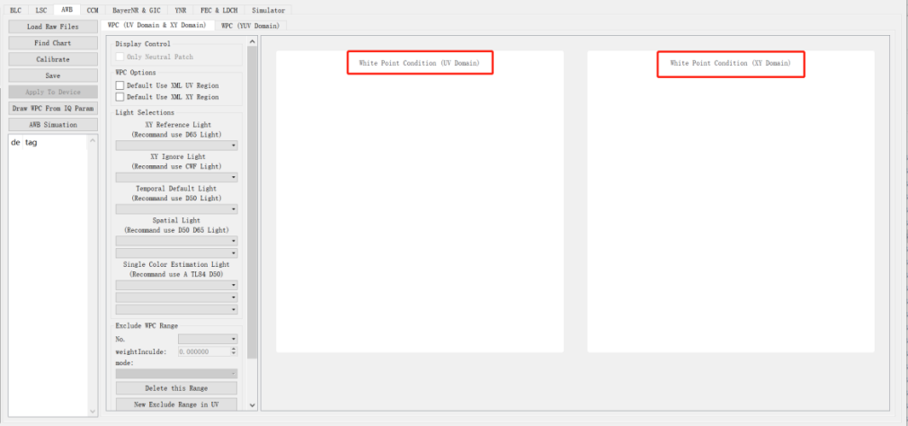
Figure 4-4-3-1
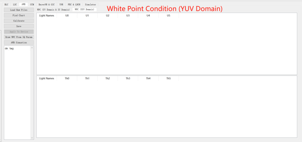
Figure 4-4-3-2
- Instructions for adjusting white point conditions in the UV and XY domains
a) Use the mouse to drag the four corners of the white point area of any light source in the coordinate system to adjust the position and size
b) Drag the mouse in the blank area in the coordinate system to adjust the display range.
c) Use the scroll wheel to zoom in and out to adjust the scale.
d) The Exclude WPC Range parameter can set the non-white point area and the extra light source white point area.
- Click the “AWB Simulation” button, this function can be used to detect the white point of the original image, calculate the WB Gain and the number of white points, and map the specified pixels to the UV and XY domains to confirm the correct white point conditions.
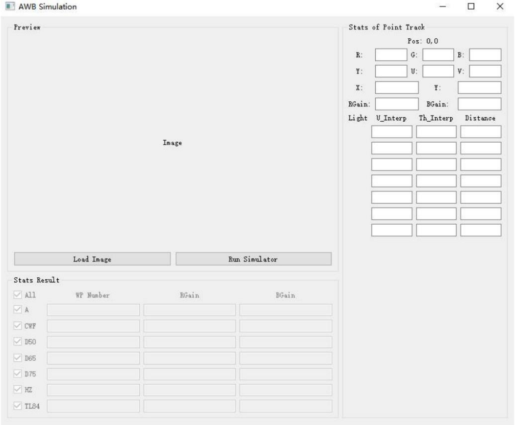
Figure 4-4-3-3
a) After clicking LoadImage to import the raw image, as shown below, the white point information will be printed. The white points of different light sources are displayed in different colors. The number of white points in the middle frame and large frame, RGain accumulation and BGain accumulation will be displayed in the three text boxes of WP Number, RGain and BGain
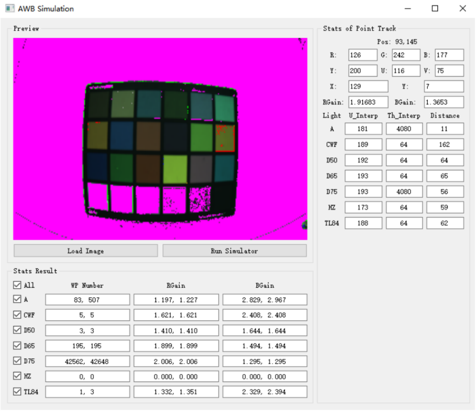
Figure 4-4-3-4
b) Click any position in the image (the black arrow as shown below), it will be mapped to the UV domain axes and the XY domain (small black square), which is convenient to check whether the point falls in the white point range. At the same time, the R G B U V X Y RGain BGain (red frame area) of the point is displayed, and the u and th after the point is mapped to each light source in the yuv domain and the deviation distance from the standard white point (corresponding to the three columns in the green frame area)
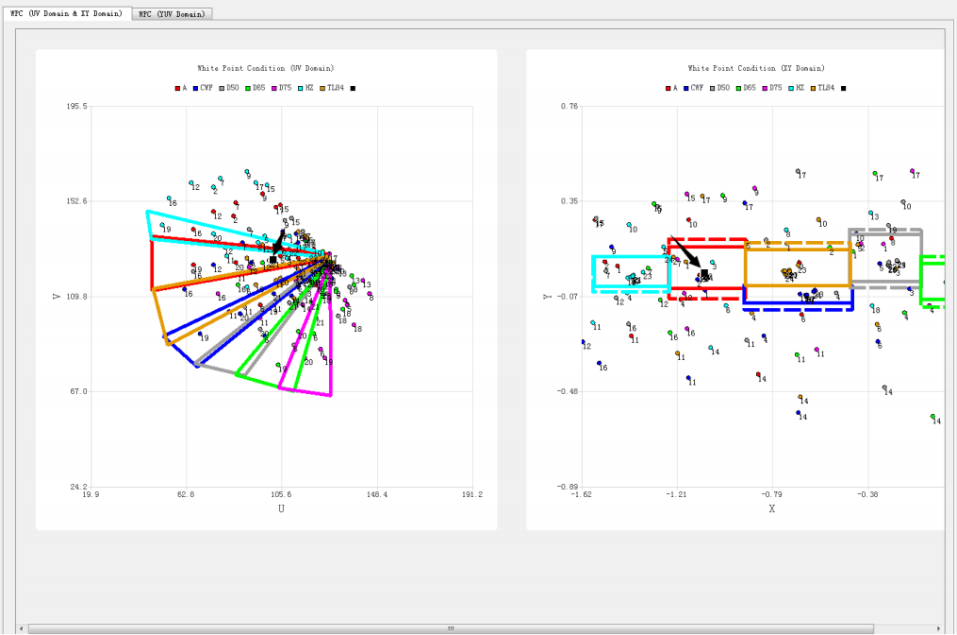
Figure 4-4-3-5
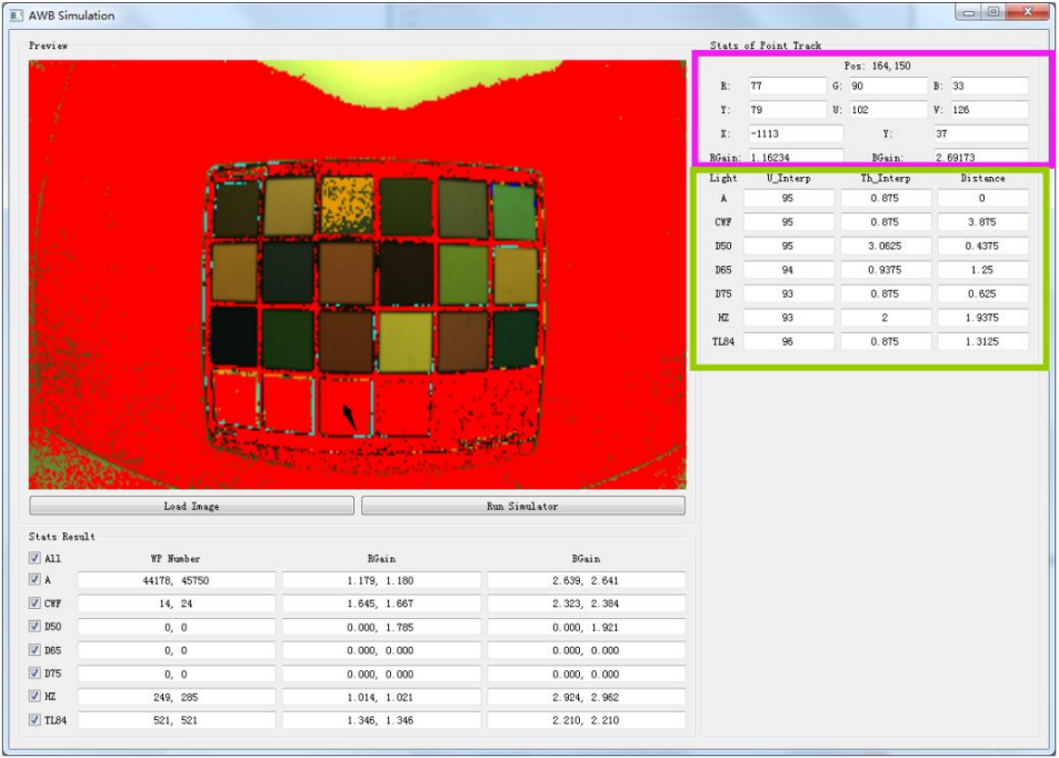
Figure 4-4-3-6
4.4.4 Calibration Procedure
- Open Calibration Tool, click Edit Options to open the configuration window, and enter the size, sensor bpp and bayer order of the raw image.
- Before AWB calibration, we must complete the BLC and LSC calibration.
- Click Load Raw Files to import the raw images of A, CWF, D50, D65, D75, HZ, TL84 (we recommend these seven light sources).
- Click Find Chart to open the color block search GUI. If the imported image is mirrored, it can be flipped through the Flip function area on the right. The current version supports horizontal and vertical flips.
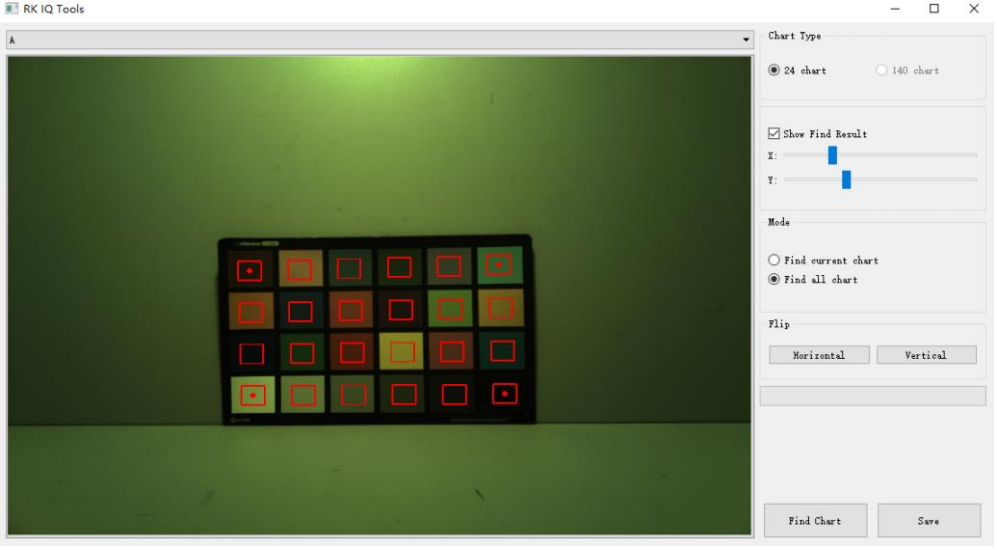
Figure 4-4-4-1
a) Adjust the statistics area by dragging the red frame center dots on the upper left, upper right, lower left and lower right, and try to ensure that the statistics area is in the center of each color block, as shown in Figure 4-4-4-1
b) Click FindChart to identify the color blocks of all light sources, as shown in Figure 4-4-4-2
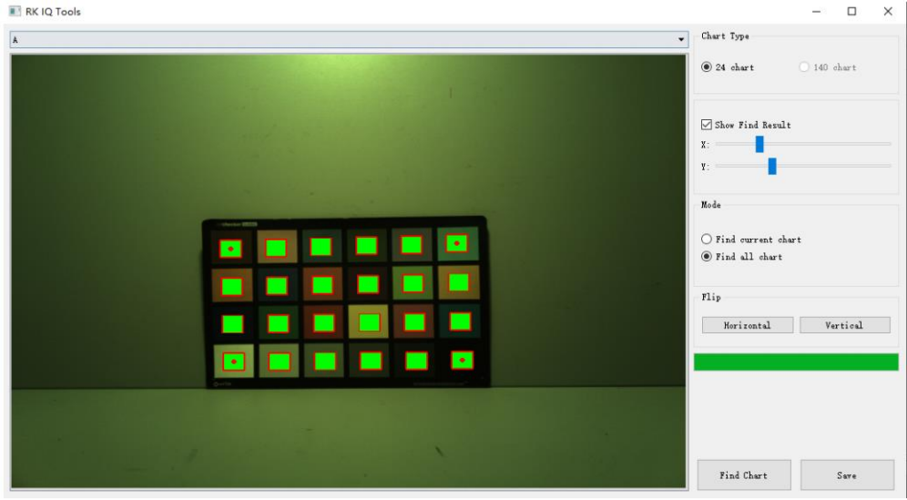
Figure 4-4-4-2
c) Select another light source from the menu to confirm that the color patch detection results are correct. If the detection is correct, as shown in Figure 4-4-4-4. If it is found that the position of the detection result is wrong, as shown in Figure 4-4-4-3, it is only necessary to re-detect it separately. Select “Find Current Chart” in Mode and repeat steps a) and b) until the detection result is correct.
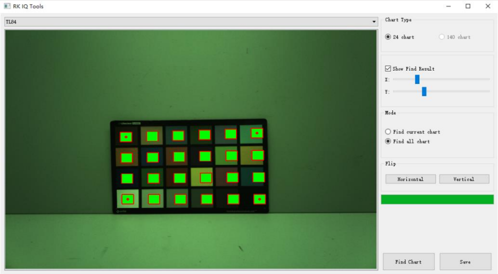
Figure 4-4-4-3
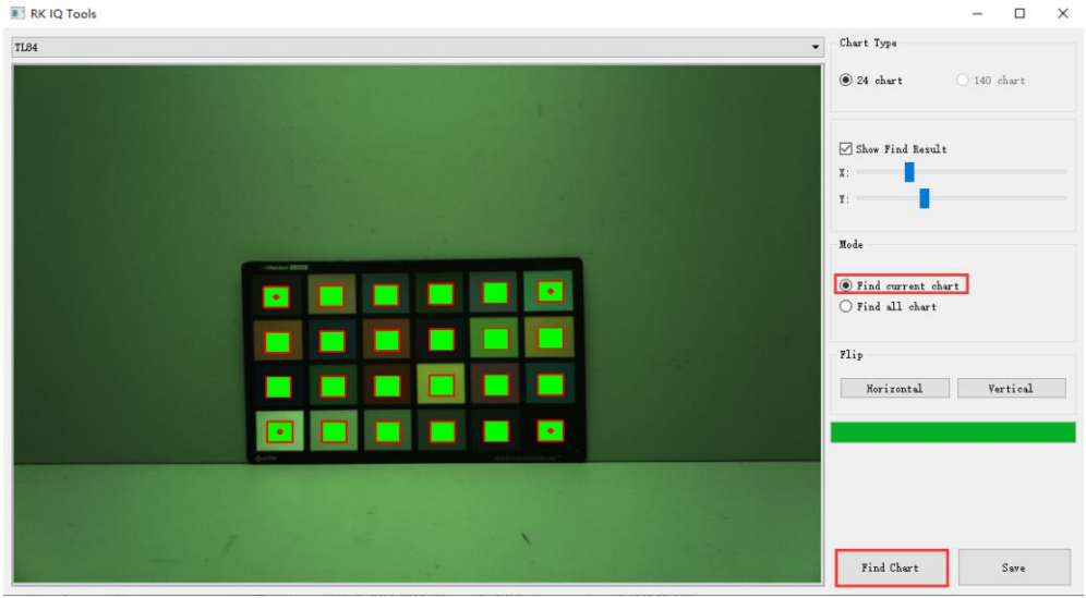
Figure 4-4-4-4
d) Click the save button to complete the detection
- Click Calibrate to start. It will take about 30s. the following initial white point conditions and other parameters are obtained. Those dots in different colors in the coordinate systems of the UV and XY domains represent the positions of the color block values in the ColorChecker captured by each light source in the UV and XY color spaces, the rectangle box represents the white point conditions of different light sources.
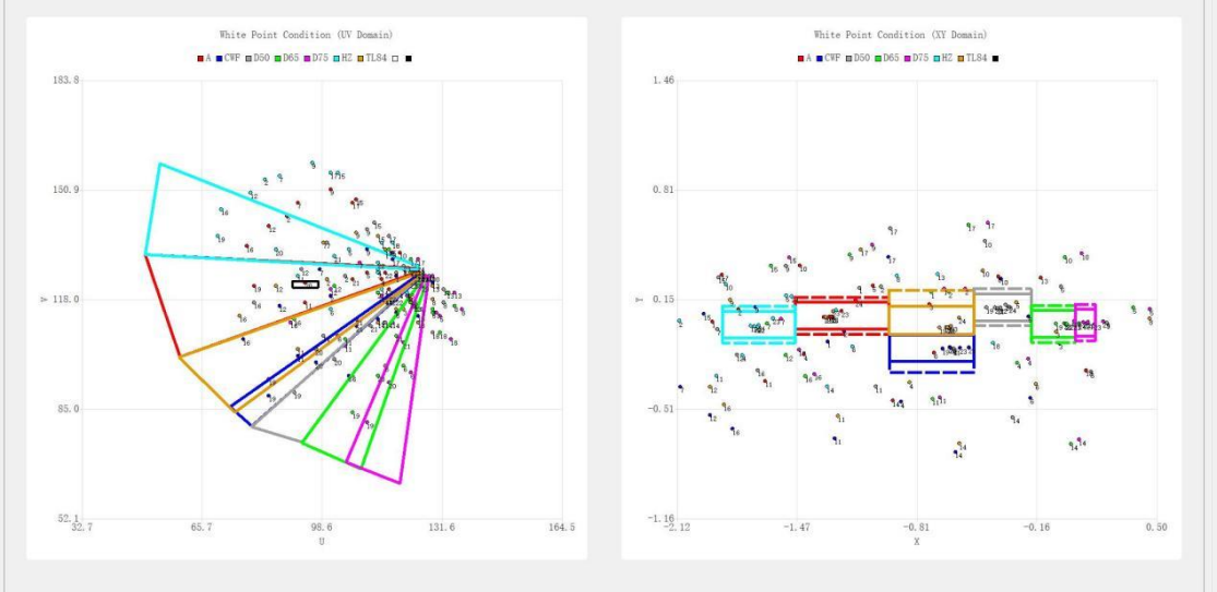
Figure 4-4-4-5
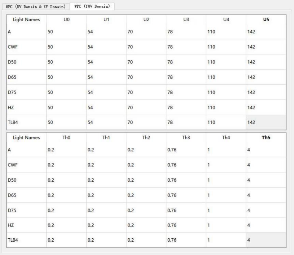
Figure 4-4-4-6
- Click AWB Simulation and import the raw images of A, CWF, D50, D65, D75, HZ, TL84 in turn to check the accuracy of white point detection.
- Modify the frame of the UV domain or the XY domain or the TH of the YUV to make the white point detection of the ColorChecker under each light source more accurate.
- Click Save, and click Run Simulator on the AWB Simulation interface to view the white point detection results of the imported light source image.
- Repeat steps 6 to 8 until the white point detection of each light source is reasonable.
Notes:
- Adjust the condition, try best to make white points (points marked 19, 20, 21, and 22 blocks) inside the box, and the non-white points are outside the box.
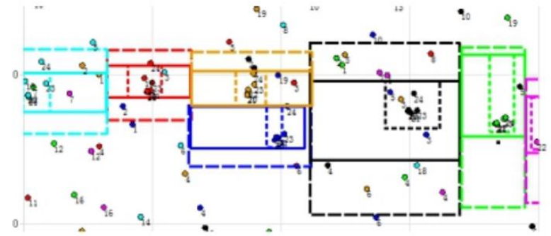
- The middle box of all light sources on the blackbody locus is continuous in the x direction. Example of error as shown in the below: Small spacing between large boxes, but large spacing between middle boxes
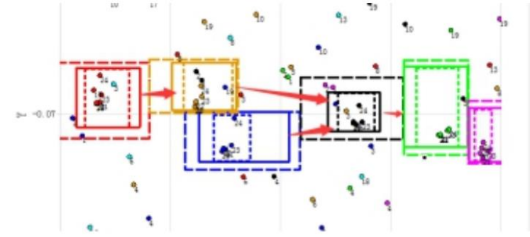
The correct example is as follows:
- A and HZ light sources can be slightly smaller in the Y direction of the XY domain, and D50 and D65 can be slightly larger in the Y direction of the XY domain.
- Two light sources with very close color temperature (CWF and TL84) can be changed to be adjacent in the Y direction.
- In the UV domain, there cannot be a gap between any two light sources.
- The areas of different light sources can overlap, but do not overlap in both the XY and UV domains at the same time.
- When excluding non-white points, adjust the UV domain with the distribution of the XY domain as a reference.
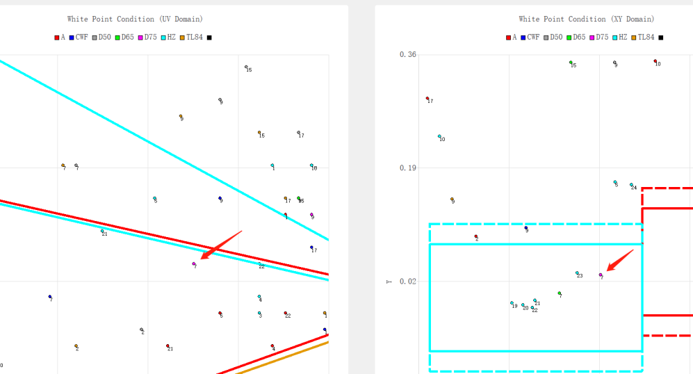
For example, the 7th block of D75 circled in the picture below falls within the HZ range and will be incorrectly detected as a white point.
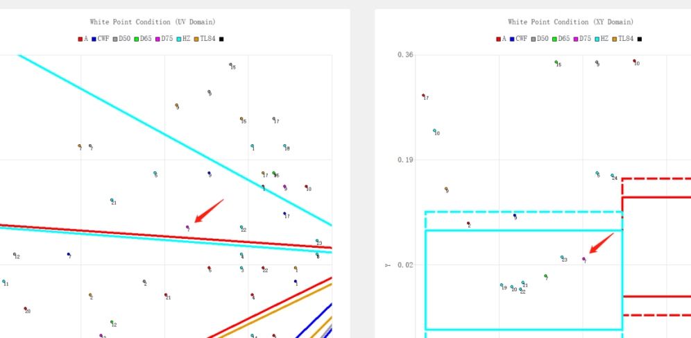
After readjustment, the 7th block of D75 light source is not in the same light source in xy and uv space and will not be recognized as a white point.
- When the non-white point falls in the white point range of XY and UV, it can also be excluded by reducing TH, or by increasing the non-white point range.
- When the white point falls within the white point range of XY and UV, but it is still not a white point, it may be excluded because it exceeds the brightness range, or it falls within the non-white point range, or it is less than TH and does not fall within the white point range. In the white point interval of the YUV domain.
4.4.5 Example of AWB Calibration Results
Final White Point Conditions:
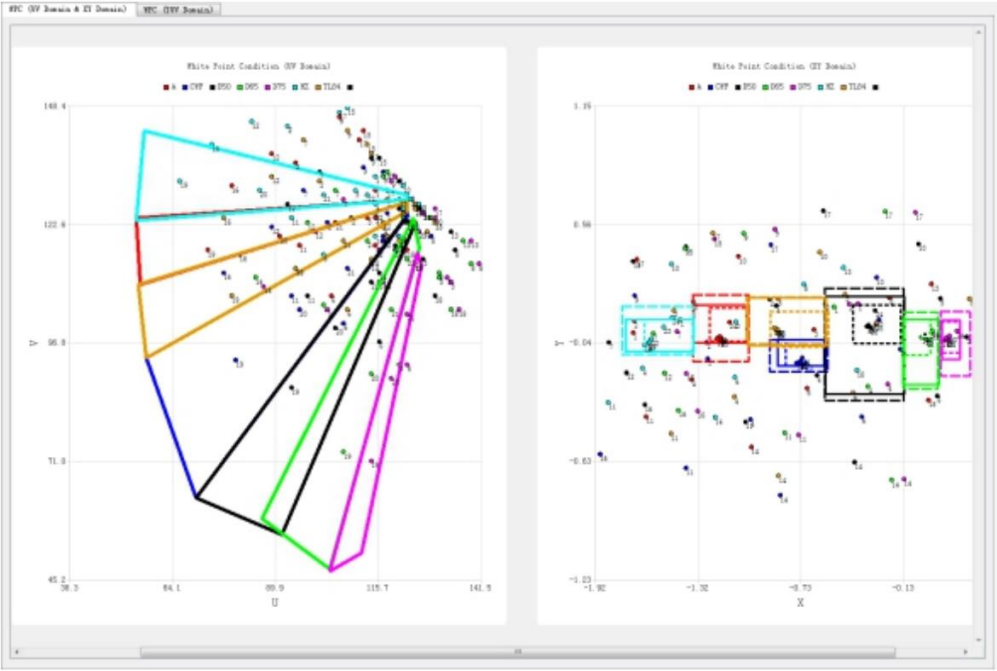
Figure 4-4-5-1
The white point detection results of each light source are:
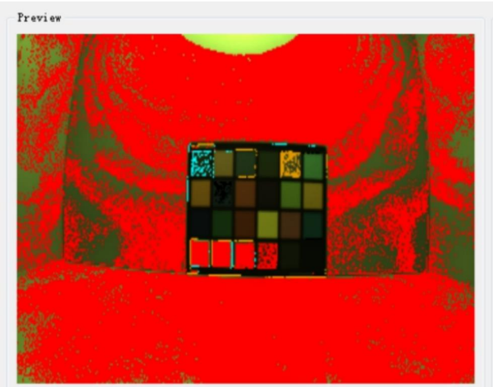
Figure 4-4-5-1 A
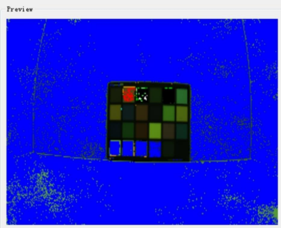
Figure 4-4-5-2 CWF
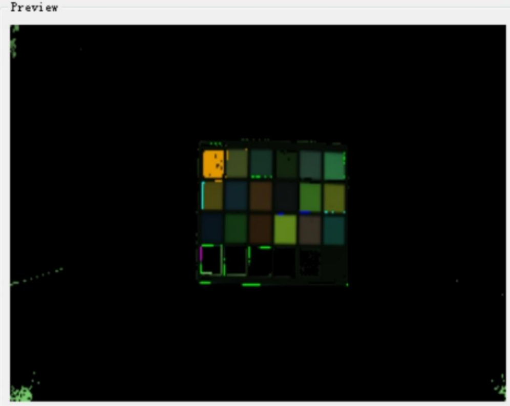
Figure 4-4-5-3 D50
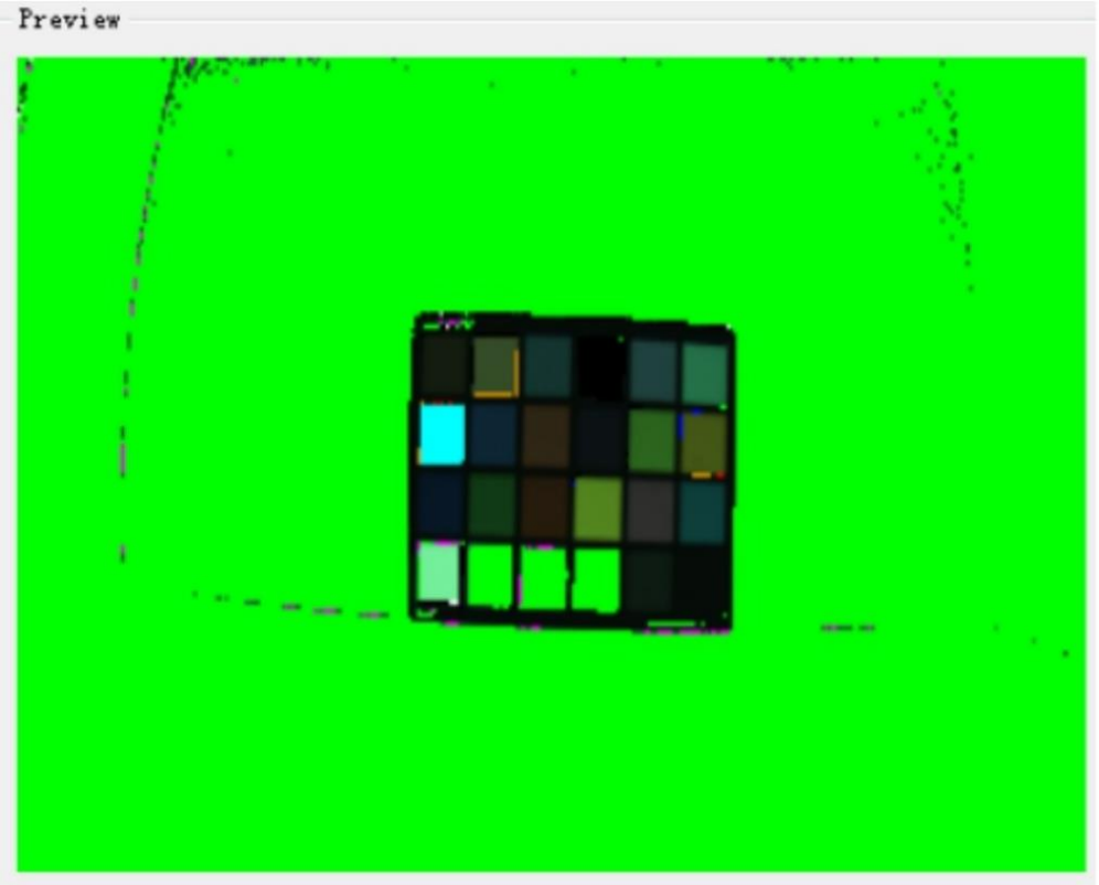
Figure 4-4-5-4 D65
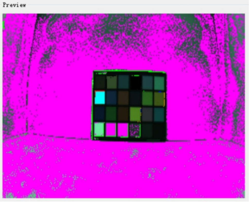
Figure 4-4-5-5 D75
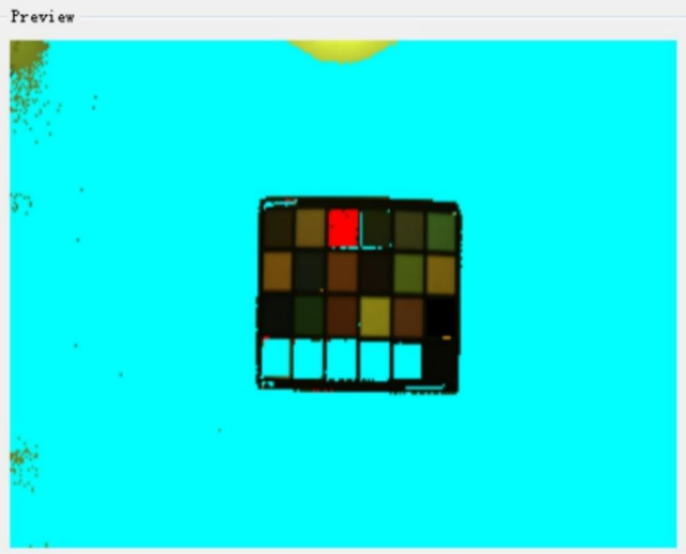
Figure 4-4-5-6 HZ
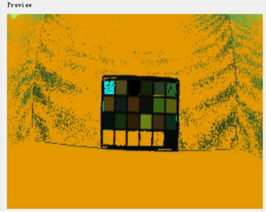
Figure 4-4-5-7 TL84
4.5 CCM Calibration
4.5.1 Raw Image Requirements
The raw image requirements refer to chapter 4.4, CCM can use the raw image of AWB to calibration. In addition, since the Gamma curve will affect the CCM results, it may be necessary to adjust the CCM parameters again when the Gamma curve is modified. In this case, please refer to chapter
4.5.2, point 12.
4.5.2 CCM Calibration Procedure
- Open the Calibration Tool, select the CCM, and click the Load Raw Files to import all raw images. The imported raw image will be displayed in the list:
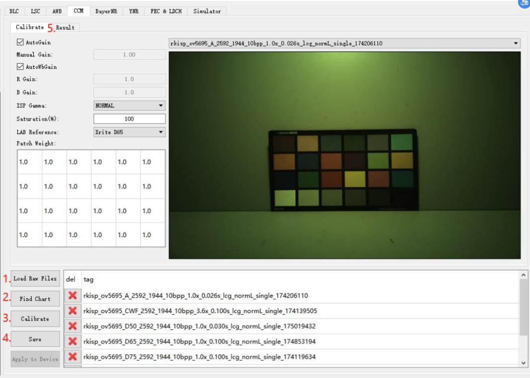
Figure 4-5-2-1
- Click Find Chart to open the color block search GUI.
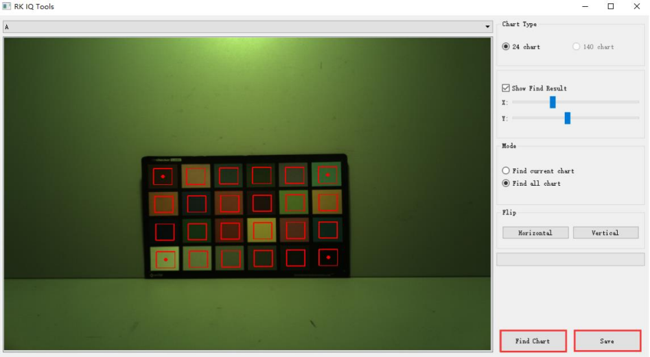
Figure 4-5-2-2
- Drag the red frame center dots on the upper left, upper right, lower left, and lower right to adjust the sampling area, and make sure that the sampling area is in the center of each color block.
- Click Find Chart to start counting the color block values, and the statistical area will be marked in green.
- Check each light source in the list and confirm whether the statistical area is correct.
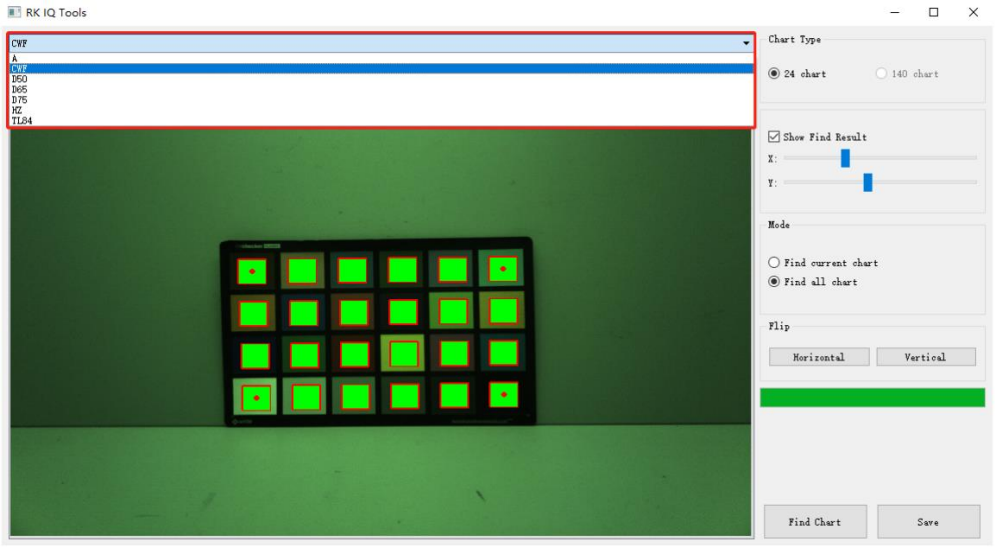
Figure 4-5-2-3
- After the search is complete, click Save and then exit.
- Set the saturation to 100%, as shown in Figure 4-5-2-4.
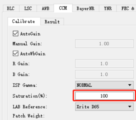
Figure 4-5-2-4
- Click the Calibrate to start the calibration. It takes about 20s.
- After the calibration is completed, the calculation result will be on the result page.
- Click the Save button.
- Modify the saturation to 74% and repeat steps 8~10.
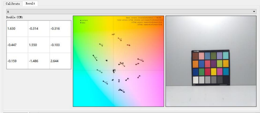
Figure 4-5-2-5
- If ΔE is too large, the raw image may be too bright. You can right-click the ColorChecker image on the right side of Figure 4-5-2-5, click Save Current, save the image, and check whether each color patch is overexposed or a certain channel is saturated (CCM calibration after applying the Gamma curve may cause calibration patches saturation).
a) If there is a problem of over-brightness or over-saturation, you should re-capture the color chart of the light source, reduce the exposure, and re-calibrate.
b) If the brightness of the color blocks is normal, the possible causes of the problem are: abnormal BLC parameters, abnormal LSC parameters, lens light leakage (infrared light), etc..
- For specific tuning methods, please refer to Rockchip_Color_Optimization_Guide
4.6 NR Calibration
4.6.1 Raw Image Requirements
NR module raw image capture instructions:
- Capture in a light box with a standard light source, it is recommended to use a DC light source with adjustable brightness.
- A grayscale gradient card must be used, as shown in Figure 4-6-1-1.
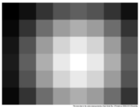
Figure 4-6-1-1
- Exposure needs to traverse Gain=1x, 2x, 4x, 8x, 16x…Max (for example, if the maximum gain is supported to 40x, then Max=32).
- Four Raw images need to be captured under each Gain, namely highlight-stacked frame, highlight-single frame, low-light-stacked frame, and low-light single frame.
- High light and low light can be distinguished by adjusting the exposure time or light brightness, and multiple frames and single frames are generated by tool processing.
- The following brightness values are all 8-bits.
- Low-light image requirements: the pixel value of the brightest block in Figure 4-6-1-1 reaches 30 (to ensure that the boundary of each color block can be seen clearly, if it is not satisfied, it can be appropriately increased), and the pixel value of the darkest block reaches Black-Level (It can be satisfied when the pixel value of the brightest block just reaches 30).
- Highlight image requirements: the pixel value of the brightest block in Figure 4-6-1-1 reaches 255, and the pixel value of the darkest block is generally around 60-70.
- RK Capture Tool provides the YNR Capture function, which can automatically search for qualified exposure combinations based on the brightness of the darkest and brightest blocks settings.
4.6.2 Capture Raw Image
- Open the RK Capture Tool, refer to the instructions in sections 3.1 and 3.2 to connect the device.
- Put the device or module in the light box, and stick the gradient chart on the light box.
- Adjust the position of the device so that the gradient chart is moved to the center of the screen, and it is as close to the picture as possible.
- Turn on the light box and switch the light source to TL84 or CWF.
- Modify the light source name to TL84 or CWF, and the module name to NR_Normal.
- Assuming that the sensor supports Gain=1-24, we need to capture 1x 2x 4x 8x 16x.
- Select the YNR Capture, first take a raw image, right-click on the preview on the right and select Draw ROI, and select the brightest block and the darkest block in the preview image in turn (represented by black and white blocks later), double-click the rectangle, we can re-draw it, fix the image position and the rectangle position, and perform NR capturing, as shown in
Figure 4-6-2-1.
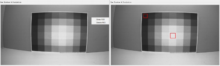
Figure 4-6-2-1
- Capturing the low-light raw image: The brightness of the light box is adjusted to about 800lux. Modify the value of Gain Range in the tool to 1.0 - 1.0, and Exp Range will not be modified. Check Multi-Frame and Low-Light. Select the YNR Capture page and fill in the thresholds of the black and white rectangles. set FrameNumber=32. Black Block Mean Luma: The target value to be achieved by the black block, which is initially filled in as BLC(8bit)+1. White Block Mean Luma: The target value to be achieved by the white block, the initial fill is
30.
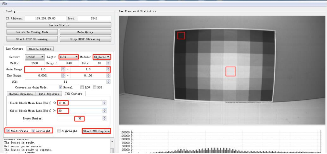
Figure 4-6-2-2
a) Click the Start YNR Capture button to start capturing, and the current average pixel value of the two rectangular boxes and the corresponding exposure parameters will be printed in the log box; meanValue[0]: the current average pixel value of the black block; meanValue[1]: The current average pixel value of the white block; blackTarget: the filled Black Block Mean Luma threshold; whiteTarget: the filled White Block Mean Luma threshold.
b) When the threshold value cannot capture the image, as shown in Figure 4-6-2-3, check the log, find that meanValue[1] is just larger than the meanValue[0] of whiteTarget, and set this value to Black Block Mean Luma (In order to avoid noise interference threshold, meanValue[0] can be slightly increased), as shown in Figure 4-6-2-4.
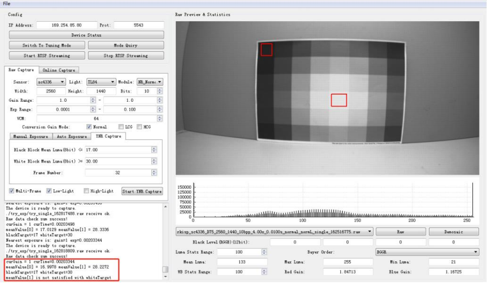
Figure 4-6-2-3
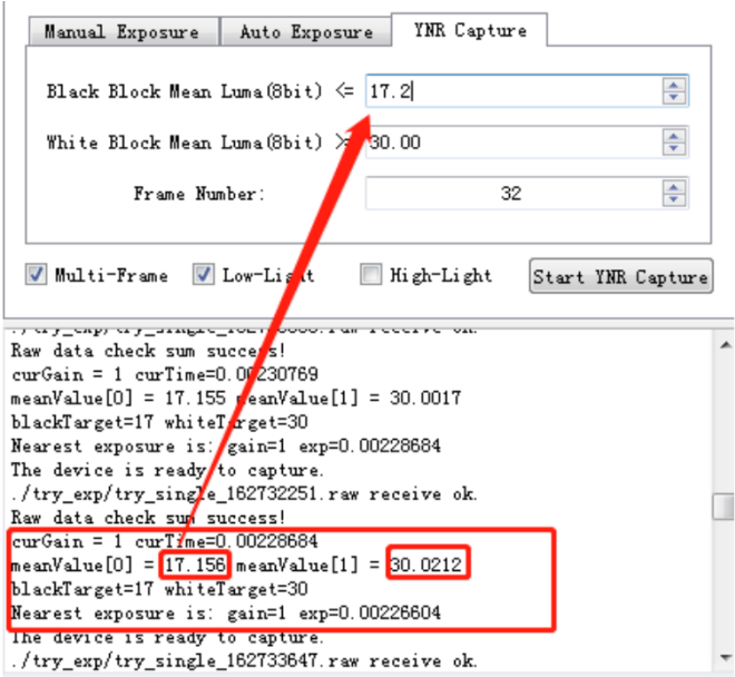
Figure 4-6-2-4
c) After finding the threshold that satisfies the conditions, click the Start YNR Capture button again to start the capture. After the capture is completed, one Raw image with the Multiple and Single suffixes is obtained, as shown in Figure 4-6-2-5.
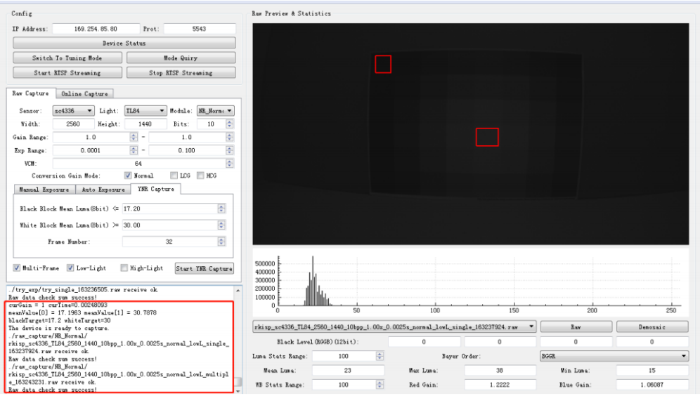
Figure 4-6-2-5
- Capturing the high-light raw image: The brightness of the light box is adjusted to about 800lux. Modify the value of Gain Range in the interface to 1.0 - 1.0, and Exp Range will not be modified. Check Multi-Frame and High-Light. Select the YNR Capture page and fill in the following two boxes for the thresholds. Black Block Mean Luma: Indicates the target value to be achieved by the darkest block, the initial fill is 60. White Block Mean Luma: Indicates the target value to be achieved by the brightest block, fixed at 255. set FrameNumber=32
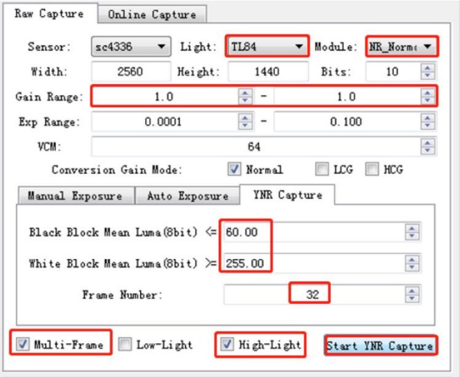
Figure 4-6-2-6
a) Click the Start YNR Capture button to start capturing, and the log of the tool will print the average value of the ROI area, exposure and gain after each exposure adjustment. meanValue[0]: the current average pixel value of the darkest block. meanValue[1]: the current average pixel value of the brightest block. blackTarget: the filled Black Block Mean Luma threshold. whiteTarget: the filled White Block Mean Luma threshold.
b) When the exposure and gain reach the maximum, but the brightness of the brightest block still cannot reach 255, as shown in Figure 4-6-2-7, you need to manually adjust the brightness of the light box, and then click Start YNR Capture to re-capture, after the conditions are met Obtain a Raw image with Multiple and Single suffixes, as shown in Figure 4-6-2-8.
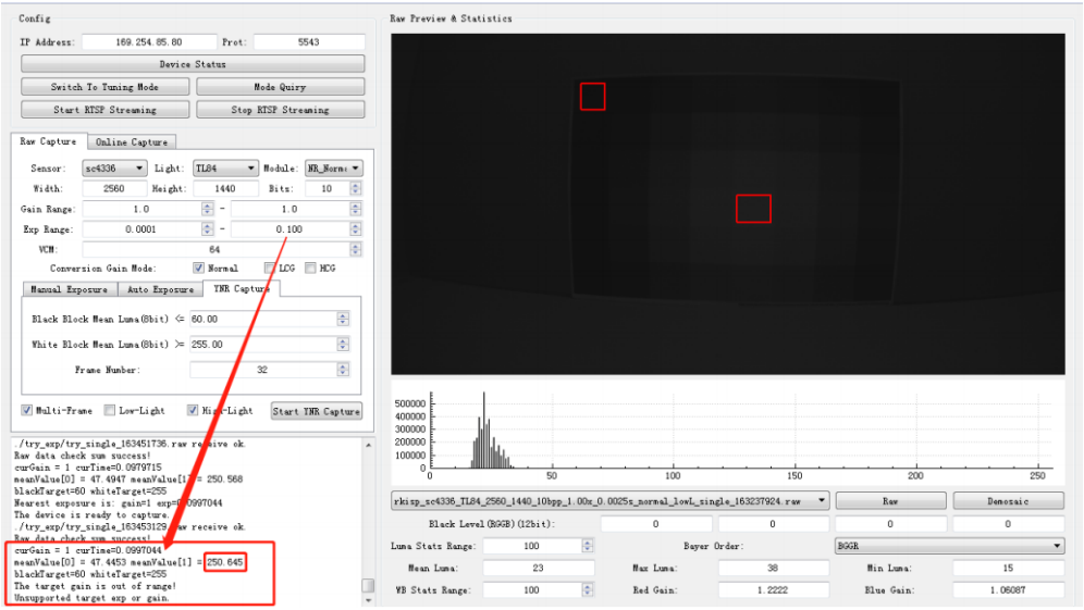
Figure 4-6-2-7
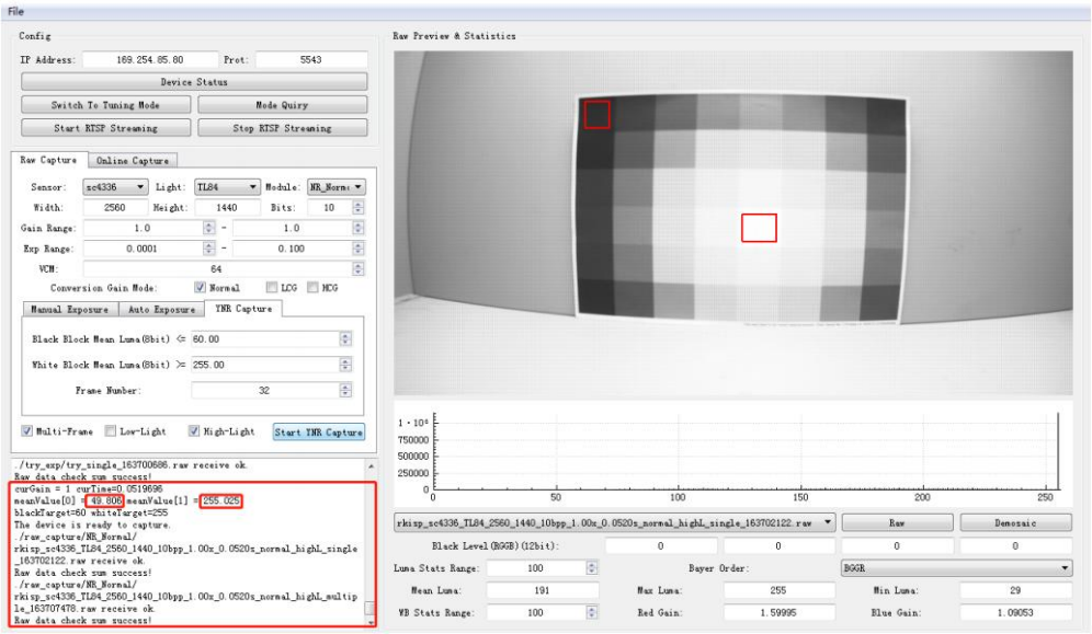
Figure 4-6-2-8
- Modify the Gain Range value to 2x, and repeat steps 8 and 9 until all Gain capturing is completed.
- Since the Gain will continue to increase, the threshold of the black block will be greatly affected by the noise, and the threshold of the black block can be slightly adjusted according to the printed log.
4.6.3 Calibration Procedure
GIC & BayerNR and YNR & MFNR modules share the same set of Raw images:
- Open Calibration Tool, click the Edit Options button in the upper left corner, enter the size, bit width and bayer order of the Raw image.
- Select the GIC & Bayer NR page, click the Load Raw Files button to import all Raw images, and the imported Raw images will be in the list below.
- Click Find ROI to frame the position of the gradient chart, as shown in Figure 4-6-3-1, make sure that the rectangular frame is within the color block.
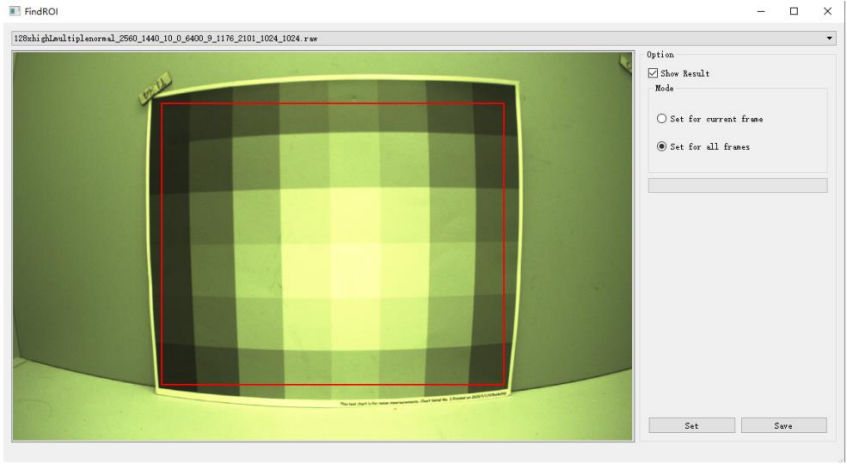
Figure 4-6-3-1
- Click Calibrate button to start.
- The BayerNR noise curve obtained after the calibration is completed will be displayed in the right window, as shown in Figure 4-6-3-2.
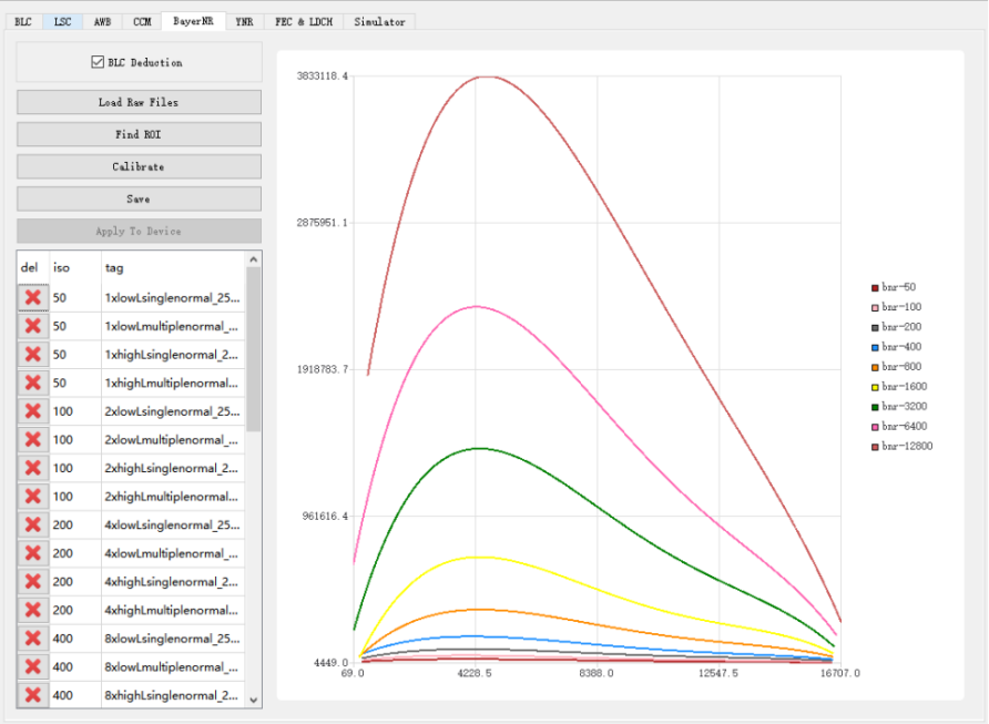
Figure 4-6-3-2
- Click Save.
- Select the YNR&MFNR page, click the Load Raw Files button to import all Raw images, and the imported Raw can be found in the list below.
- Click the Calculate YUV button, the Raw image will be processed into a YUV image by the simulator.
- Click the Calibrate button, and check YNRCurve Print before Calibrating to save the calibration parameters and sampling points of each iso.
- The YNR noise curve obtained from calibration will be in the right window, as shown in Figure 4-6-3-3.
- Click Save.
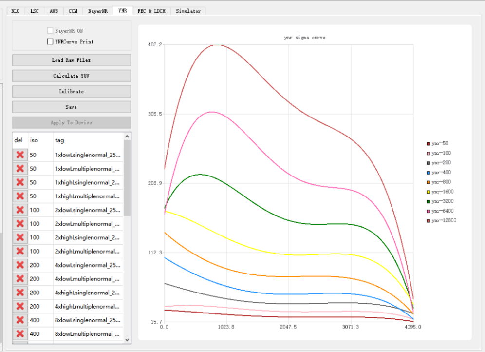
Figure 4-6-3-3
Notes: If the generated noise curve is very different from the curve in Figure 4-6-3-3, it may be that the high light or low light brightness is wrong. You can judge according to the abnormal position of the curve: The wrong curve on the left means that the low light brightness is not suitable. The wrong curve on the right means that the highlight brightness is not suitable. The color temperature of the light source used should not be too high or too low, otherwise the result of Calculate YUV may be incorrect. If the minimum brightness of the light box cannot meet the capturing requirements, you can use a light reduction film to assist the capture.
4.7 FEC/LDCH
To use the FEC/LDCH module, a map table is needed. The map table only with the coordinates of the horizontal x/y direction of the image, and is a mapping table after down-sampling. To get the map table, we need to know the relevant parameters of the camera lens. We need to capture a set of checkerboard images, and then use the calibration tool to calibrate.
4.7.1 Calibration Image Requirements
Capturing checkerboard, the checkerboard size is changeable, and the calibration image only supports jpg, bmp, png format. Checkerboard capturing has two modes: Method 1: One image contains only one checkerboard (higher precision, recommended). Method 2: One image contains n checkerboards (for the convenience of calibration, n=4).
- Preparations (1) The checkerboard should be a standard calibration board. If you print the checkerboard by yourself, please pay attention to the real size. The self-printed checkerboard should have a flat surface, preferably fixed on a flat board. The number of checkerboards grids should be different from the horizontal and vertical grids as much as possible, which is convenient for the calibration tool to identify the direction. (2) Appropriate lighting conditions and capturing environment: The lighting is moderate to ensure that the images from all angles during the capturing process are clear, and there should be no reflection or blur on the checkerboard. In the whole process, the aperture and focal length of the camera should be fixed, and it is necessary that the amount of light entering the camera and the focal length are fixed.
- Operating rules (1) Appropriate ratio: try to make the captured checkerboard image occupy between 1/4 and 1/8 of the entire camera field of view. (2) Appropriate number: make sure that the checkerboards of all images can cover the entire camera field of view, the number is usually about 15, too few quantities will cause inaccurate calibration parameters. It is recommended to take 3-4 pictures at the same position, In order to facilitate subsequent screening and replacement of unqualified images. (3) Appropriate distribution: As shown in Figure 2-1, make sure that the captured images of the calibration board are evenly distributed in all areas and corners of the camera’s field of view, and when it is close to the edge of the field of view, the checkerboard should be as close to the edges as possible, but take care that do not make the checkerboard out of the image field of view. (4) Different tilt angles: We should not just capture images parallel to the plane of the lens, but make sure it with different tilt angles.
- Capturing demonstration
There are two ways to capture: (1) Method 1 (recommended) Four calibration pictures, the checkerboard occupies four positions of the upper left, upper right, lower left and lower right in the calibration picture, and there is no specific order.
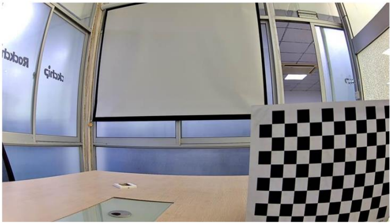
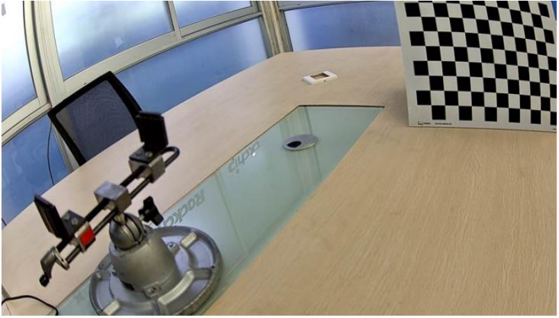
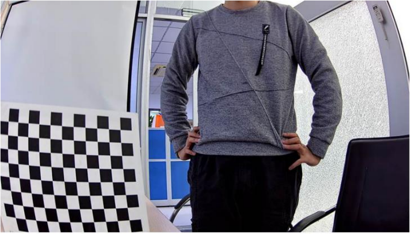
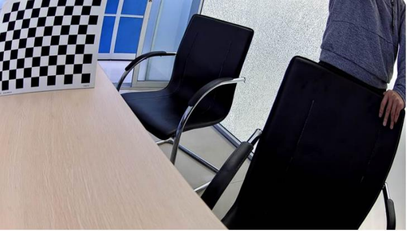
Figure 4-7-1-1
(2) Method 2 A calibration image, the upper left, upper right, lower left and lower right corners are covered with checkerboards.
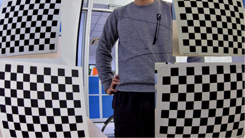
Figure 4-7-1-2
4.7.2 Calibration Procedure
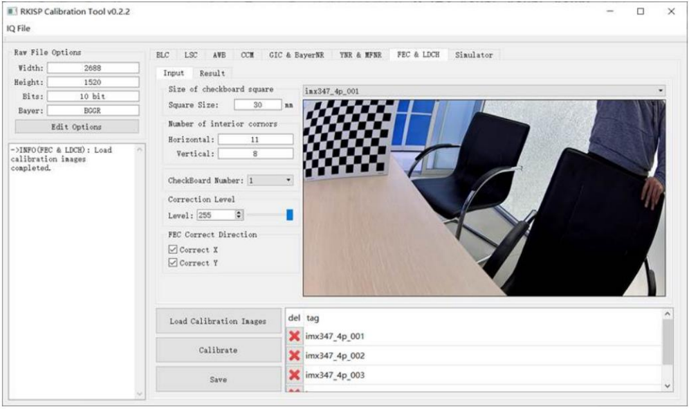
Figure 4-7-2-1
- Configure the resolution in the Raw Options. Bit and Bayer Pattern can be ignored.
- Import the folder of calibration images. Support jpg, bmp, png formats.
- Adjust the calibration configuration parameters.
a) Square Size: The actual size of each grid in the checkerboard, generally 30mm or 25mm.
b) Horizontal/Vertical: The number of inner corner points of the horizontal (Horizontal) and vertical (Vertical) of the checkerboard:
c) Check Board Number: the number of checkerboards in each image can be 1 or 4.
d) Level: Set the Level of distortion correction, which is divided into 256 levels. Level = 0 means that the mapping table obtained at this time has no correction effect (that is, the output image is the same as the input image), and Level = 255 means that the mapping table is the maximum degree of correction that LDCH can achieve.
e) Correct Direction: If the mapping table is generated for the FEC module, we can also set different corrections: i. Only check Correct X: Only correct the horizontal direction, the effect is similar to LDCH. ii. Only check Correct Y: only the vertical direction is corrected. iii. Both Correct X and Correct Y: both horizontal and vertical directions are corrected.
- Click Calibrate.
- Save the results.
How to distinguish the corners and interior corners of the checkerboard (see Figure 4-7-2-2). The picture below shows a checkerboard with 12 horizontal and 9 vertical grids. The number of horizontal corners is 13, the number of horizontal inner corners is 11, and so on. So Horizontal = 11, Vertical = 8.
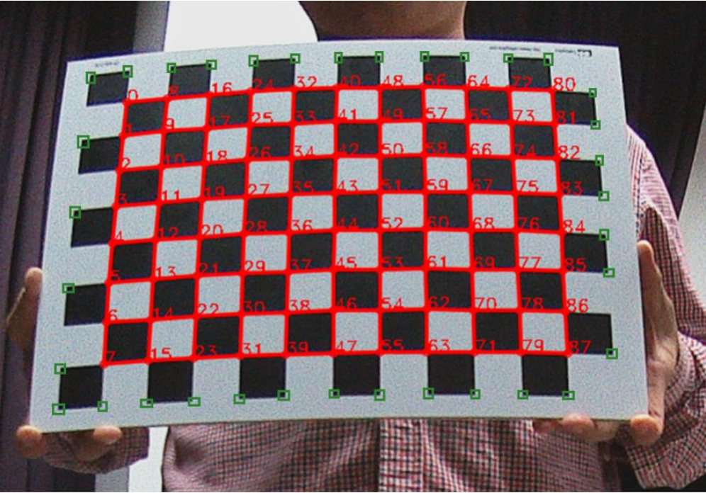
Figure 4-7-2-2 The corners and interior corners of the checkerboard
(Corners include red and green parts, while inner corners only include red parts)
Notes:
- Check the “result” folder exists in the toolpath, if not, we have to create a new folder called “result” and place it in the same directory as the Calibration Tool.
- The outermost circle of the chessboard is indeed calculated. However, when capturing the image, the black and white blocks in the outermost circle cannot be completely blocked by the preview.
- The number of corner points in the horizontal direction is equal to: the number of black and white blocks in the horizontal direction minus 1.
- The number of corner points in the vertical direction is equal to: the number of black and white blocks in the vertical direction minus 1.
- FEC is corrected in both directions by default. When calibrating, the direction can be selected.
- The folder for storing the image, preferably named after sensor name + lens name/focal length + resolution, the tool will generate a folder for storing calibration files according to this name
4.7.3 Example of Calibration Results
- If there is an unsuccessful calibration result, generally, the corner detection is inaccurate or incomplete due to the unclear capturing of the checkerboard. Therefore, we should first check whether the corners of each image checkerboard are completely and accurately detected, and the number of complete detections cannot be less than 3.
- If the calibration is successful, the result shown in Figure 4-7-3-1 will appear. We can view the calibrated distortion parameters in the “log” on the left. The meanings of the six parameters from top to bottom are: the center coordinates of the camera (cx, cy), camera distortion parameters (a0, a2, a3, a4).
- On the “result”, we can view the checkerboard corner detection results for each image. If the detection result is inaccurate, delete the image, and re-calibrate it to obtain a more accurate result. The generated FEC and LDCH mapping table is stored in the corresponding folder under the “result”.
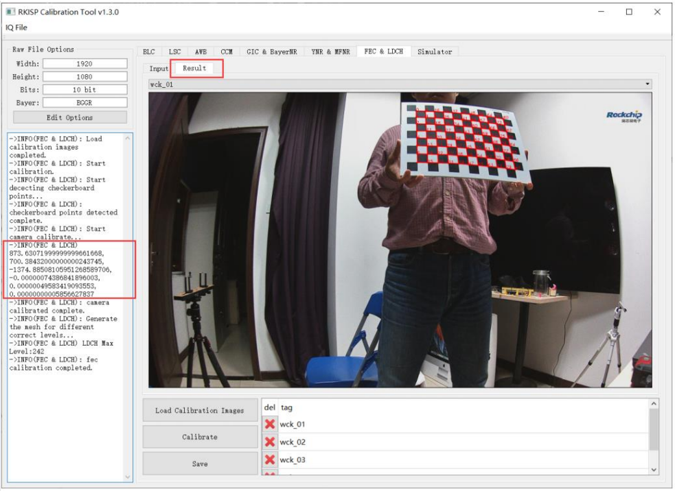
Figure 4-7-3-1
5 Online Tuning
5.1 Introduction of Tuning GUI
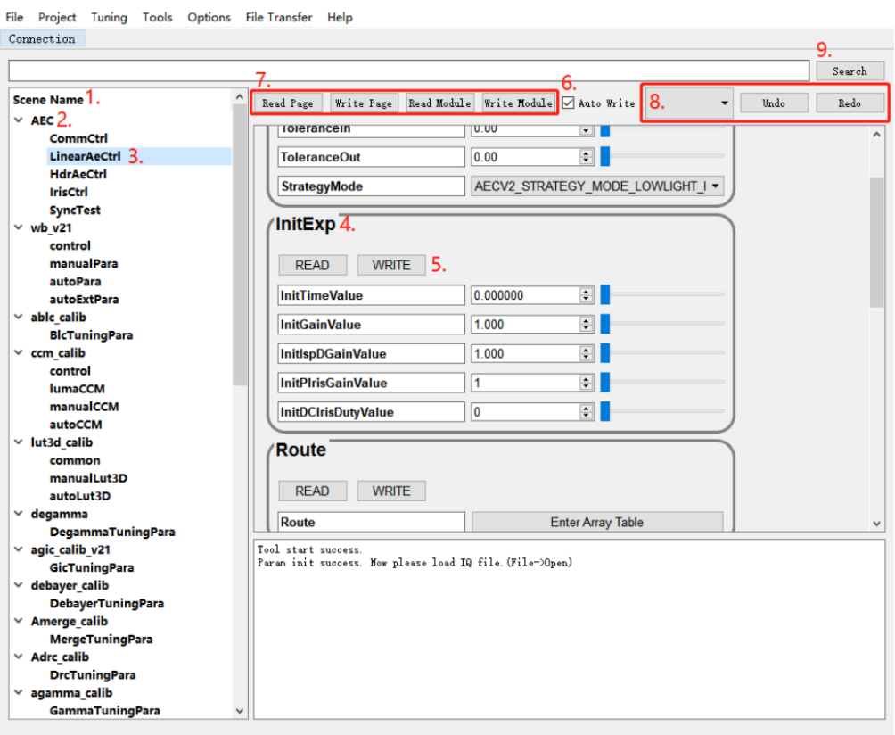
Figure 5-1-1 Main UI of RKISP Tuner v2
As shown in Figure 5-1-1, this interface is a typical state of use: the interface after the loading and tuning UI is completed and the IQ parameters are imported. The following briefly introduces the UI meaning and functions of the numbers marked in the figure:
- Module tree structure diagram: “normal: day” displayed at the top is the name of the scene selected to load when loading IQ parameters, where “normal” is the name of the main scene, and day is the name of the sub-scene.
- ISP module: a scene can contain multiple modules, and a module can contain some pages.
- Tuning page: A module node can contain multiple tuning pages, and a tuning page can contain some tuning units.
- Tuning unit: For example, the unit name is InitExp, which contains 5 numeric member parameters.
- Tuning unit read and write buttons: provide online read and write functions for all parameters in the entire unit.
- Automatic writing function: when it is checked, if the tool has been connected to rkaiq_tool_server, every parameter modification will be automatically sent to the device and the settings will take effect.
- Page/module read/write button: provide online read and write functions for the entire page or module.
- Undo/Redo function: Can undo the last modification operation, if AutoWrite is checked, the device will also synchronize the operation.
- Search function: find the page where the parameter is located according to the keyword.
5.2 Platform & Network Configuration Function
Open the platform & network configuration window when you start the tool for the first time or click the “Project” - “Network and Platform Settings” button in the menu bar, as shown in the following figure
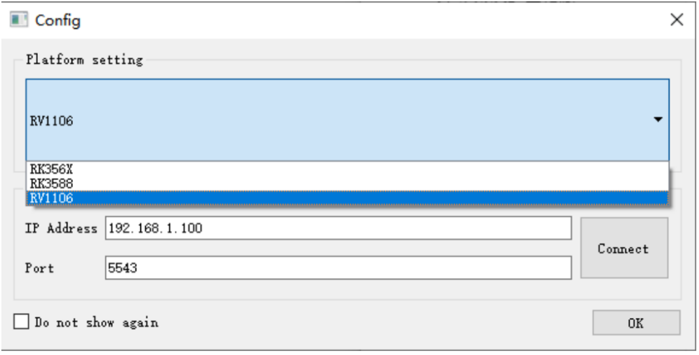
Figure 5-2-1
1.Platform Setting: Selecting the chip will load different configuration files of tuning UI. The correspondence between different platforms and configuration files is recorded in config/config.ini
- Network Config: Configure the network address of the device, the port number is 5543 by default, do not modify it unless there are special requirements
Click the “Connect” button, the tool will try to establish a connection to the rkaiq_tool_server in the device, please make sure rkaiq_tool_server is running correctly
5.3 Registers and Algorithm Parameters
Each tuning unit contains registers or algorithm parameters. According to the different parameter forms and value ranges, different controls are used, which generally have the following four categories:
- Numerical value: an integer or floating-point value with a certain range of values. Modify the value directly Use the up and down arrows to adjust the value Use the slider on the right to adjust the value
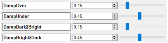
Figure 5-3-1
- Boolean: a parameter whose value is 0 or 1, mainly for various function switches, etc.. Take 1 when Enable, and take 0 when Disable.

Figure 5-3-2
- List: choose one of the preset options, mainly for various function modes, ISO, Day/Night and LCG/HCG gear selection.

Figure 5-3-3
- Table: NxM matrix parameters, the matrix elements may be integer or float, expand by clicking the “Show data” or “Enter Array Table” on the tuning unit.
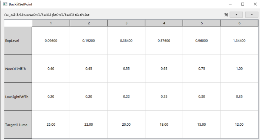
Figure 5-3-4
5.4 Online Tuning of Gamma Parameters
5.4.1 Gamma Visual Tuning
- As shown in Figure 5-4-1-1, enter the GammaTuningPara page, and click the “Edit Curve” of the Gamma_Curve parameter to open the Gamma visual tuning UI
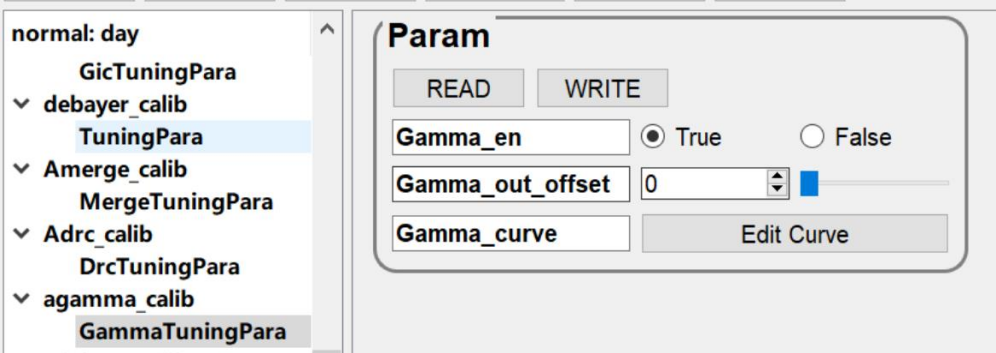
Figure 5-4-1-1 Gamma UI
- As shown in Figure 5-4-1-2, the Gamma visual tuning UI includes the following functions:
1) Curve adjustment area: Drag the red dot with mouse to adjust the curve. When AutoWrite is checked, each adjustment will be set to the board end in real time.
2) Curve Coeff: Supports generating Gamma curves based on coefficients. Note that the curves corresponding to the coefficients will be automatically generated after modification here, and the curves originally adjusted manually may be overwritten.
- Position Control: move the mouse on the dot, the coordinates will be updated to the X and Y boxes, we can manually set the Y value of the point.
- Control Point Number: Adjust the number of control points, support four types (49, 45, 24, 13).
- Axis Range: Adjust the scale of the coordinate axis, both X and Y axes support adjustment, mainly used for adjustment of denser areas in dark area nodes.
- Export/Import: Supports exporting Gamma curves as files to save or reading Gamma curves from files.
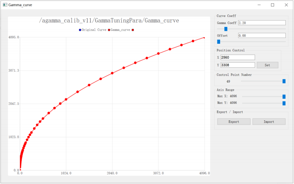
Figure 5-4-1-2 Gamma visual tuning window
5.4.2 Tuning Method of Gamma Curve
There are two curves on the axes, the blue one is the original curve, the red one is the current adjustment curve, when the pointer moves to the dot on the red curve, it will be displayed as up and down arrows, you can drag the dot to move up and down, The red curve will change with the position of the point, as shown in Figure 5-4-2-1.
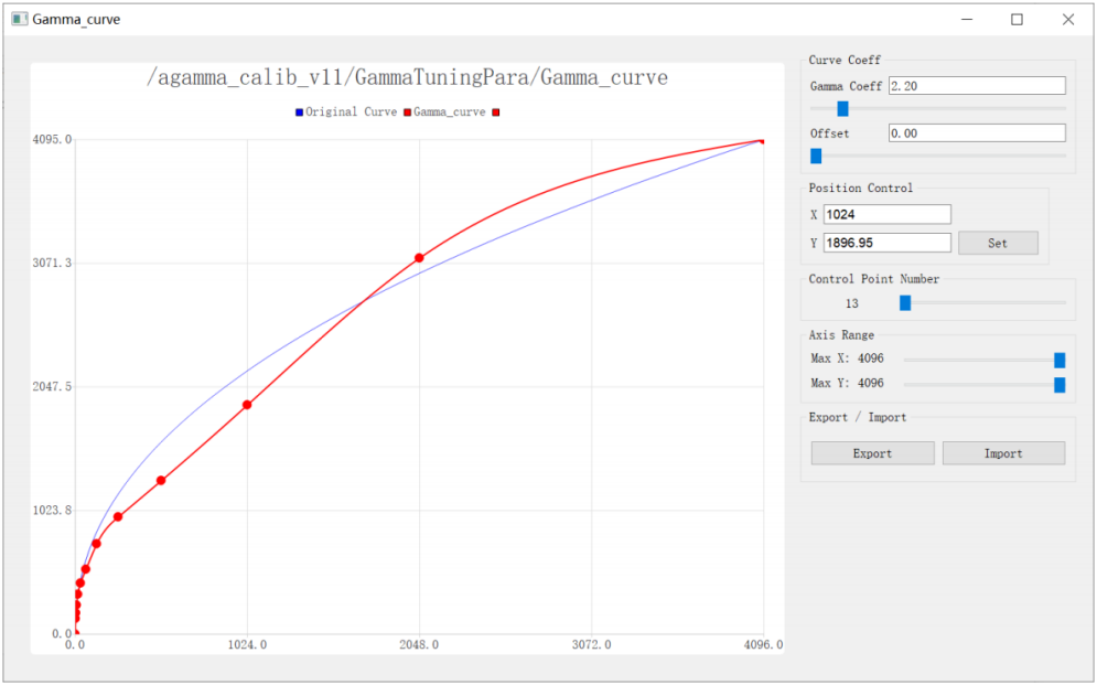
Figure 5-4-2-1 The curve after dragging the dot
Modify the “Gamma Coeff” in Curve Coeff to 1.5 and press “Enter”, a new curve will be generated according to the coefficient, as shown in Figure 5-4-2-2
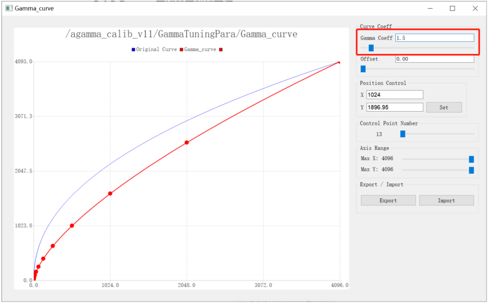
Figure 5-4-2-2 Generate Curves Using Coefficients
6 Other functions
6.1 IQ File Import Function
Click “File Transfer” - “Send File To Device” in the menu bar, select the IQ file to be transferred, and enter the path to save the IQ file on the device, as shown in Figure 6-1-1, click “Send”, after the transfer complicated, the file can be found in the target path.
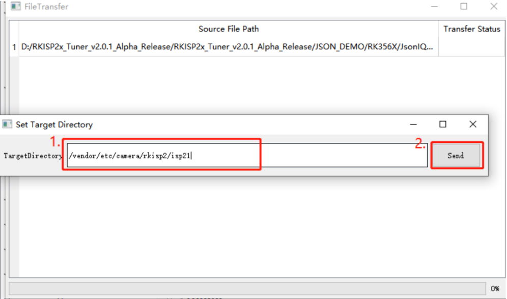
Figure 6-1-1 Set Transferring Path
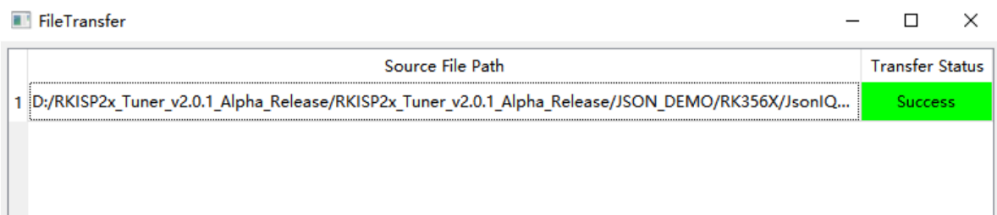
Figure 6-1-2 File Transfer Success
6.2 Offline Raw Simulation
This function is used to import the raw image back to the board, and run the ISP to process it.
- Click “File - Send RAW Image To Device” to open the configuration window
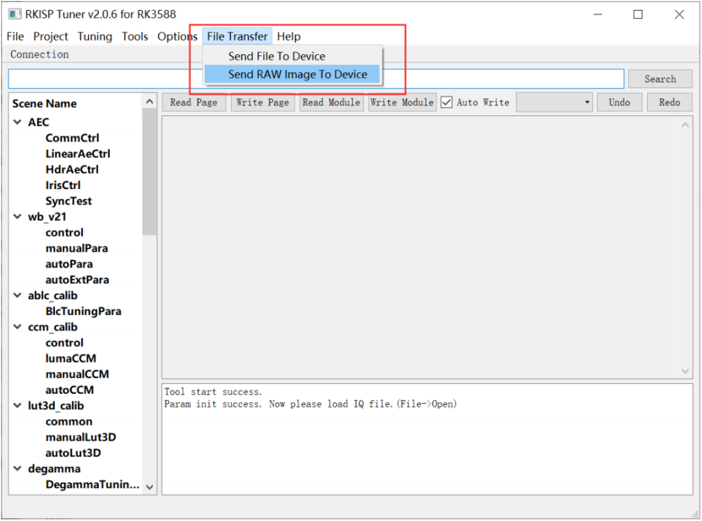
Figure 6-2-1 Open the Raw configuration page
- Click “Add” to load the raw files
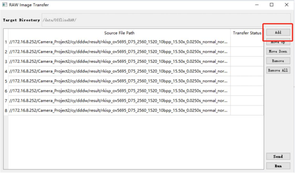
Figure 6-2-2 Load Raw image
Note: This function only support “.rkraw” format, and the internal data is “compact+align256”. Other formats can be converted in batches using RKRAW Tool. Please also configure “RKRawV2” in “config.ini” to 1 when capture Raw. (For the method of Online Capture of Raw, please refer to the description in Section 3.7.2)
- Click “Send” the Raw image to the device, and this will generate a configuration file under “/tmp”
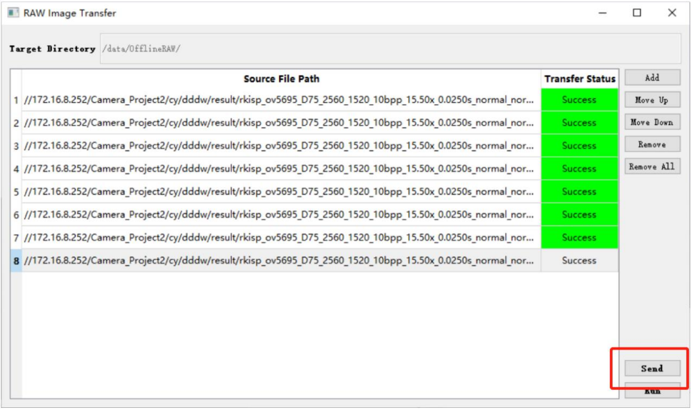
Figure 6-2-3 Send Raw image to the device
- Don’t close this window and restart the camera app. After the device detects the configuration file, it will switch to the offline simulation mode.
- Click “Run” to start simulation process.
- The raw images are sent to the ISP one by one and the processed images can be seen in the preview of the camera app. In this state it supports: online tuning parameter reading and writing, and capture YUV images.
- If you need to replace the raw file, refer to the following process:
1) Click Stop to pause the offline simulation.
2) Click Add to load the raw files.
3) Click Send to send the raw files.
4) Click Run to start the offline simulation.